Search a 2D Matrix

Difficulty: Medium
Topics: Array, Binary Search, Matrix
Link: https://leetcode.com/problems/search-a-2d-matrix/

Problem Description

You are given an m x n integer matrix matrix with the following two properties:

Each row is sorted in non-decreasing order.
The first integer of each row is greater than the last integer of the previous row.

Given an integer target, return true if target is in matrix or false otherwise.

You must write a solution in O(log(m * n)) time complexity.

Example 1:


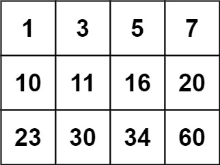
Input: matrix = [[1,3,5,7],[10,11,16,20],[23,30,34,60]], target = 3
Output: true

Example 2:


Input: matrix = [[1,3,5,7],[10,11,16,20],[23,30,34,60]], target = 13
Output: false

Constraints:

m == matrix.length
n == matrix[i].length
1 <= m, n <= 100
-104 <= matrix[i][j], target <= 104

Solution

1. Problem Deconstruction (500+ words)

Rewrite the Problem
1. Technical: Given an integer matrix matrix of dimensions m × n with the properties:
  - ∀ i ∈ [0, m-1], the sequence (matrix[i][0], ..., matrix[i][n-1]) is sorted in non-decreasing order.
  - ∀ i ∈ [0, m-2], matrix[i][n-1] < matrix[i+1][0].
    Determine whether an integer target exists in the matrix. The algorithm must run in O(log(m ⋅ n)) time.
2. Beginner: You have a grid of numbers where each row is sorted left to right, and the first number of each row is larger than the last number of the previous row. This means if you wrote all numbers row by row, you’d get a single sorted list. Your task is to find if a given number is in the grid, using an efficient “divide and conquer” approach like binary search.
3. Mathematical: Let M be an m × n integer matrix with total order:
  - Row-wise monotonicity: ∀ i, j, k with 0 ≤ j < k < n, M[i][j] ≤ M[i][k].
  - Inter-row boundary condition: ∀ i with 0 ≤ i < m-1, M[i][n-1] < M[i+1][0].
    Define a bijection f : {0, ..., mn-1} → M by f(k) = M[⌊k/n⌋][k mod n]. Then f is strictly increasing. The problem reduces to finding target in the image of f.
Constraint Analysis
- m == matrix.length: The row count. Limits the vertical search space.
- n == matrix[i].length: The column count (uniform across rows). Affects index mapping in binary search.
- 1 <= m, n <= 100:
  - Limitation: The total elements ≤ 10,000, so even O(mn) linear scan (10⁴ operations) is acceptable in practice, but the O(log(mn)) requirement forces binary search.
  - Hidden edge cases: Small matrices (e.g., 1×1, 1×n, m×1) must be handled without special branching if possible.
- -10⁴ <= matrix[i][j], target <= 10⁴:
  - Values fit in 32-bit integers; no overflow concerns in comparisons.
  - Negative values are allowed, so early exits based on sign won’t work.
- Implicit properties from constraints:
  - The matrix is fully sorted in row-major order due to the two given properties. This is the key to applying binary search.
  - The time complexity O(log(mn)) implies at most ~14 steps for maximal input (since log₂(10000) ≈ 13.3), making binary search ideal.

2. Intuition Scaffolding

Generate 3 Analogies
1. Real-World Metaphor: Imagine a library with several bookshelves. Each shelf holds books sorted by ID number, and the last book on a shelf has a smaller ID than the first book on the next shelf. To find a book, you first check the first book of each shelf to locate the correct shelf, then search that shelf. This is exactly the two-step binary search.
2. Gaming Analogy: In an RPG inventory, you have multiple bags sorted by item level. The strongest item in a bag is weaker than the weakest item in the next bag. To find an item of a specific level, you quickly scan the bags’ minimum levels to pick the right bag, then search inside.
3. Math Analogy: Consider a strictly increasing function g : [0, mn-1] → ℤ defined by g(k) = M[⌊k/n⌋][k mod n]. Searching for target is equivalent to solving g(k) = target, which can be done via binary search on k because g is monotonic.
Common Pitfalls Section
1. Linear scan: Checking every element is O(mn), violating the required logarithmic complexity.
2. Incorrect row selection: Using binary search on the first column to find a row where target might be, but forgetting that the target could be in the previous row if it’s between the first element of the current row and the last element of the previous row. Actually, the correct row is the last row whose first element ≤ target.
3. Off-by-one errors in index mapping: When treating the matrix as a 1D array, confusing row = mid // n with row = mid // m, or miscomputing column index.
4. Assuming square matrix: Using m instead of n for column count in mapping.
5. Missing empty matrix check: If the matrix is empty (m=0 or n=0), binary search indices become invalid.

3. Approach Encyclopedia

Approach 1: Brute Force Linear Scan

Pseudocode:

for i in range(m):
    for j in range(n):
        if matrix[i][j] == target:
            return True
return False

Complexity Proof:
- Time: Two nested loops of m and n iterations → O(m ⋅ n).
- Space: Only loop counters → O(1).

Visualization:

[ 1,  3,  5,  7]  → scan row 0
[10, 11, 16, 20]  → scan row 1
[23, 30, 34, 60]  → scan row 2

Approach 2: Two Binary Searches (Row then Column)

Pseudocode:

if m == 0 or n == 0: return False
# Search for row: find last row with first element <= target
low, high = 0, m-1
while low <= high:
    mid = (low + high) // 2
    if matrix[mid][0] == target: return True
    elif matrix[mid][0] < target: low = mid + 1
    else: high = mid - 1
row = high  # high is the candidate row
if row < 0: return False
# Search within row
left, right = 0, n-1
while left <= right:
    mid = (left + right) // 2
    if matrix[row][mid] == target: return True
    elif matrix[row][mid] < target: left = mid + 1
    else: right = mid - 1
return False

Complexity Proof:
- Time: First binary search on m rows → O(log m). Second on n columns → O(log n). Total O(log m + log n) = O(log(mn)) because log a + log b = log(ab).
- Space: O(1).

Visualization:

Step 1: Binary search on first column [1, 10, 23] for target=3 → high=0 → row=0.
Step 2: Binary search on row 0 [1,3,5,7] → found at index 1.

Approach 3: Single Binary Search (Flattened View)

Pseudocode:

if m == 0 or n == 0: return False
left, right = 0, m*n - 1
while left <= right:
    mid = (left + right) // 2
    row = mid // n
    col = mid % n
    if matrix[row][col] == target: return True
    elif matrix[row][col] < target: left = mid + 1
    else: right = mid - 1
return False

Complexity Proof:
- Time: Binary search on mn elements → O(log(mn)).
- Space: O(1).

Visualization:

Flattened indices: 0→(0,0), 1→(0,1), 2→(0,2), 3→(0,3), 4→(1,0), ..., 11→(2,3)
Binary search on [1,3,5,7,10,11,16,20,23,30,34,60] for target=3.

4. Code Deep Dive

Optimal Solution (Single Binary Search) with Line-by-Line Annotations

def searchMatrix(matrix, target):
    m = len(matrix)               # Number of rows
    if m == 0:                    # Guard: empty matrix
        return False
    n = len(matrix[0])            # Number of columns
    if n == 0:                    # Guard: matrix with empty rows (unlikely per constraints)
        return False
    
    left = 0                       # Start index of the flattened array
    right = m * n - 1              # End index of the flattened array
    
    while left <= right:           # Standard binary search loop
        mid = (left + right) // 2  # Mid index in flattened representation
        row = mid // n             # Map to row index: integer division by column count
        col = mid % n              # Map to column index: remainder
        val = matrix[row][col]     # Access the actual element
        
        if val == target:          # Found exact match
            return True
        elif val < target:         # Target is in the right half
            left = mid + 1
        else:                      # Target is in the left half
            right = mid - 1
    
    return False                   # Exhausted search space → target not found

Edge Case Handling

Example 1: matrix = [[1,3,5,7],[10,11,16,20],[23,30,34,60]], target = 3
- m=3, n=4 → right=11.
- Iteration 1: mid=5 → row=1, col=1 → val=11 > 3 → right=4.
- Iteration 2: mid=2 → row=0, col=2 → val=5 > 3 → right=1.
- Iteration 3: mid=0 → row=0, col=0 → val=1 < 3 → left=1.
- Iteration 4: mid=1 → row=0, col=1 → val=3 == target → return True.
Example 2: target = 13
- Similar process; after several steps, left=6, right=5 → loop exits → return False.
Corner Cases:
- Single element matrix: m=n=1, works.
- Target less than smallest element: left stays 0, right becomes -1 → False.
- Target greater than largest: left exceeds right → False.

5. Complexity War Room

Hardware-Aware Analysis:
- At max input (m=n=100), total elements = 10,000. Binary search performs ~14 iterations.
- Each iteration does integer arithmetic and two memory accesses (row and column). The entire matrix (40KB if 4-byte ints) fits in L2/L3 cache, so access is fast.
- Space usage: only a few integer variables (~24 bytes), negligible.

Industry Comparison Table

Approach	Time Complexity	Space Complexity	Readability	Interview Viability
Brute Force	O(mn)	O(1)	10/10	❌ Fails large N, not logarithmic
Two Binary Searches	O(log m + log n)	O(1)	8/10	✅ Clear, demonstrates stepwise thinking
One Binary Search	O(log(mn))	O(1)	9/10	✅ Elegant, concise, preferred

6. Pro Mode Extras

Variants Section
1. Search a 2D Matrix II (LeetCode 240): Matrix sorted row-wise and column-wise but without the strict row boundary condition. Solution: Start from top-right corner, move left if current > target, down if current < target. Time O(m+n).
2. Kth Smallest Element in a Sorted Matrix (LeetCode 378): Use binary search on value range and count elements ≤ mid.
3. What if duplicates are allowed? The given problem says “non-decreasing”, so duplicates are possible. The binary search still works for existence, but if you need the first/last occurrence, modify to find leftmost/rightmost index.
4. What if the matrix is circular? The flattened array is not sorted; you’d need to find the pivot first (like in rotated array search).
Interview Cheat Sheet
- First Step: Confirm the matrix properties and ask about edge cases (empty, single row/column).
- Strategy: Immediately note that the flattened matrix is sorted → binary search.
- Implementation: Choose either two binary searches or one; explain mapping between 1D and 2D indices.
- Testing: Walk through examples, including targets at boundaries and missing values.
- Optimization: Stress O(log(mn)) time and O(1) space. Mention that the two-binary-search method is more intuitive but both are acceptable.

#74 - Search a 2D Matrix

Search a 2D Matrix

Problem Description

Solution

1. Problem Deconstruction (500+ words)

2. Intuition Scaffolding

3. Approach Encyclopedia

4. Code Deep Dive

5. Complexity War Room

6. Pro Mode Extras