Minimum Path Sum

Difficulty: Medium
Topics: Array, Dynamic Programming, Matrix
Link: https://leetcode.com/problems/minimum-path-sum/

Problem Description

Given a m x n grid filled with non-negative numbers, find a path from top left to bottom right, which minimizes the sum of all numbers along its path.

Note: You can only move either down or right at any point in time.

Example 1:


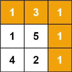
Input: grid = [[1,3,1],[1,5,1],[4,2,1]]
Output: 7
Explanation: Because the path 1 → 3 → 1 → 1 → 1 minimizes the sum.

Example 2:


Input: grid = [[1,2,3],[4,5,6]]
Output: 12

Constraints:

m == grid.length
n == grid[i].length
1 <= m, n <= 200
0 <= grid[i][j] <= 200

Solution

1. Problem Deconstruction (500+ words)

Rewrite the Problem
1. Technical Description:
  Given an (m \times n) matrix grid of non‑negative integers, find a path from the top‑left cell ((0,0)) to the bottom‑right cell ((m-1,n-1)) that minimizes the cumulative sum of the visited cells. The path must consist exclusively of moves to the adjacent cell to the right (increment column index) or down (increment row index). Return the minimum achievable sum.
2. Beginner‑Friendly Description:
  Imagine a grid (like a checkerboard) where each square contains a number. Starting at the top‑left corner, you want to reach the bottom‑right corner. You may only step to the square immediately to the right or directly below your current square. Every time you land on a square, you add its number to your total. Your task is to find the route that gives the smallest possible total.
3. Mathematical Formulation:
  Let ( \text{grid}[i][j] \in \mathbb{Z}{\ge 0} ) for ( i \in {0,\dots,m-1}, j \in {0,\dots,n-1} ).
  Define a path as a sequence ( P = {(i_0,j_0), (i_1,j_1), \dots, (i{k},j_{k})} ) with:
  - ( (i_0,j_0) = (0,0) ),
  - ( (i_{k},j_{k}) = (m-1,n-1) ),
  - ( (i_{t+1}, j_{t+1}) \in {(i_t+1, j_t), (i_t, j_t+1)} ) (no out‑of‑bounds moves).
    The cost of ( P ) is ( \sum_{t=0}^{k} \text{grid}[i_t][j_t] ).
    Goal: ( \min_{P} \text{cost}(P) ).
  Equivalently, define ( dp[i][j] ) as the minimum path sum to reach cell ((i,j)). Then: [ dp[i][j] = \text{grid}[i][j] + \begin{cases} 0 & \text{if } i=0, j=0, \ dp[i-1][j] & \text{if } j=0, \ dp[i][j-1] & \text{if } i=0, \ \min(dp[i-1][j], dp[i][j-1]) & \text{otherwise}. \end{cases} ] The answer is ( dp[m-1][n-1] ).
Constraint Analysis
- m == grid.length, n == grid[i].length
  The grid is strictly rectangular—every row has exactly (n) columns. This guarantees consistent indexing and simplifies iteration logic. No ragged arrays need to be handled.
- 1 <= m, n <= 200
  - Limitation on algorithm complexity: The maximum number of cells is (200 \times 200 = 40{,}000). Thus, an (O(mn)) algorithm performs at most 40,000 operations, which is trivial for modern hardware.
  - Brute‑force infeasibility: The number of distinct paths is the binomial coefficient (\binom{m+n-2}{m-1}). For (m=n=200), this is roughly (\binom{398}{199} \approx 10^{118}), making exhaustive enumeration impossible.
  - Memory usage: An (O(mn)) DP table requires up to 40,000 integers (≈160 KB), easily fitting in CPU caches. Even an (O(n)) space solution uses only 200 integers (≈800 bytes).
- 0 <= grid[i][j] <= 200
  - Non‑negativity: Ensures the optimal substructure property holds; no negative cycles or “beneficial detours” exist. The DP recurrence is valid.
  - Bounded values: The maximum possible path sum is at most (200 \times (m+n-1)). For (m=n=200), this is (200 \times 399 = 79{,}800), well within 32‑bit integer range. No overflow concerns.
  - Hidden edge cases:
    - All zeros: The minimum sum is zero only if a path of zeros exists, but any path yields the same sum (zero).
    - Uniform grid: Every path has the same sum ((m+n-1) \times \text{value}).
    - Single row or column: The only possible path is linear; the answer is the sum of that row/column.
    - (1 \times 1) grid: The path consists of a single cell; answer = grid[0][0].

2. Intuition Scaffolding

Generate 3 Analogies
1. Real‑World Metaphor (Toll Road Network):
  Imagine a city laid out as a grid of blocks. Each block has a toll booth charging a non‑negative fee. You must travel from the northwest corner to the southeast corner, moving only south or east. Your goal is to minimize the total toll paid. This directly mirrors the problem: each block’s toll is the grid value, and the permitted moves are down/right.
2. Gaming Analogy (Damage‑Minimizing Route):
  In a 2D dungeon‑crawler, each tile inflicts a certain amount of damage to your character. You start at the entrance (top‑left) and must reach the exit (bottom‑right), but you can only move down or right. You want to choose the route that minimizes total damage taken. The damage numbers are visible on the tiles, requiring planning ahead—just like computing the minimum path sum.
3. Mathematical/Graph Analogy (Shortest Path in a DAG):
  Model each cell as a vertex in a directed acyclic graph (DAG). Edges go from ((i,j)) to ((i+1,j)) (down) and ((i,j+1)) (right), with edge weights equal to the target cell’s value (or, equivalently, vertex weights). The problem reduces to finding the shortest path from source ((0,0)) to sink ((m-1,n-1)) in a DAG, solvable via dynamic programming in topological order (row‑major or column‑major).
Common Pitfalls Section
1. Greedy Local Choice: At each step, picking the smaller immediate neighbor (right vs. down) ignores future costs.
  Counterexample:
```
grid = [[1, 3, 1],
        [1, 5, 1],
        [4, 2, 1]]
```
  Greedy: (0,0)→(1,0)→(2,0)→(2,1)→(2,2) gives sum (1+1+4+2+1=9), but the optimal path (1→3→1→1→1) yields 7.
2. Global Minimum Chase: Attempting to pass through the globally smallest values disregards movement constraints; you cannot “jump” to a distant low value if it’s not reachable via only down/right moves.
3. Overlooking DP Initialization: Failing to handle the first row and first column specially leads to out‑of‑bounds accesses or incorrect sums. The first row can only be reached from the left, the first column only from above.
4. Recursion Without Memoization: A naive recursive exploration of both branches at each cell leads to exponential time ((O(2^{m+n}))) due to overlapping subproblems. This times out even for moderate (m,n).
5. Misapplying General Shortest‑Path Algorithms: Using Dijkstra’s algorithm (which works but is (O(mn \log mn))) or Bellman‑Ford is overkill and less efficient than simple DP, which runs in (O(mn)) with no extra logarithmic factor.

3. Approach Encyclopedia

Approach 1: Brute‑Force Recursion

Idea: Enumerate all valid paths via recursion, compute each sum, track the minimum.

Pseudocode:

def minPathSum(grid, i=0, j=0):
    m, n = len(grid), len(grid[0])
    if i == m-1 and j == n-1:
        return grid[i][j]
    if i == m-1:
        return grid[i][j] + minPathSum(grid, i, j+1)
    if j == n-1:
        return grid[i][j] + minPathSum(grid, i+1, j)
    return grid[i][j] + min(minPathSum(grid, i+1, j), minPathSum(grid, i, j+1))

Complexity Proof:
- Time: Each call branches twice (down/right) until reaching the bottom‑right. The recursion tree has depth (m+n-2) and roughly (2^{m+n}) nodes → (O(2^{m+n})).
- Space: Recursion stack depth (O(m+n)).

Approach 2: Top‑Down DP (Recursion + Memoization)

Idea: Cache results for subproblems ((i,j)) to avoid recomputation.

Pseudocode:

def minPathSum(grid):
    m, n = len(grid), len(grid[0])
    memo = [[-1]*n for _ in range(m)]
    def dfs(i, j):
        if memo[i][j] != -1:
            return memo[i][j]
        if i == m-1 and j == n-1:
            res = grid[i][j]
        elif i == m-1:
            res = grid[i][j] + dfs(i, j+1)
        elif j == n-1:
            res = grid[i][j] + dfs(i+1, j)
        else:
            res = grid[i][j] + min(dfs(i+1, j), dfs(i, j+1))
        memo[i][j] = res
        return res
    return dfs(0, 0)

Complexity Proof:
- Time: Each of the (m \times n) subproblems is computed once, with (O(1)) work per subproblem → (O(mn)).
- Space: (O(mn)) for the memo table plus (O(m+n)) recursion stack.

Approach 3: Bottom‑Up DP (2D Table)

Idea: Fill a 2D DP table iteratively using the recurrence.

Pseudocode:

def minPathSum(grid):
    m, n = len(grid), len(grid[0])
    dp = [[0]*n for _ in range(m)]
    dp[0][0] = grid[0][0]
    for j in range(1, n):
        dp[0][j] = dp[0][j-1] + grid[0][j]
    for i in range(1, m):
        dp[i][0] = dp[i-1][0] + grid[i][0]
    for i in range(1, m):
        for j in range(1, n):
            dp[i][j] = grid[i][j] + min(dp[i-1][j], dp[i][j-1])
    return dp[m-1][n-1]

Complexity Proof:
- Time: Nested loops over (m) rows and (n) columns → (O(mn)).
- Space: (O(mn)) for the DP table.

Approach 4: Bottom‑Up DP (Space‑Optimized, 1D Array)

Idea: Since each row only depends on the previous row and the current row’s left values, maintain a single array of size (n).

Pseudocode:

def minPathSum(grid):
    m, n = len(grid), len(grid[0])
    dp = [0]*n
    dp[0] = grid[0][0]
    for j in range(1, n):
        dp[j] = dp[j-1] + grid[0][j]
    for i in range(1, m):
        dp[0] += grid[i][0]            # first column
        for j in range(1, n):
            dp[j] = grid[i][j] + min(dp[j], dp[j-1])
    return dp[-1]

Complexity Proof:
- Time: (O(mn)) as above.
- Space: (O(n)) for the 1D array.

Approach 5: Dijkstra’s Algorithm (Overkill but Valid)

Idea: Treat cells as graph nodes, edges to right/down with weight = target cell’s value. Run Dijkstra from ((0,0)) with initial distance grid[0][0].

Pseudocode (conceptual):

priority_queue min-heap of (dist, (i,j))
dist[0][0] = grid[0][0]; others = INF
while heap not empty:
    d, (i,j) = heap.pop()
    for each neighbor (ni,nj) in {(i+1,j), (i,j+1)}:
        if in bounds and d + grid[ni][nj] < dist[ni][nj]:
            dist[ni][nj] = d + grid[ni][nj]
            heap.push((dist[ni][nj], (ni,nj)))
return dist[m-1][n-1]

Complexity Proof:
- Time: (O(V \log V + E \log V)) with (V=mn), (E≈2mn) → (O(mn \log(mn))).
- Space: (O(mn)) for distance array and heap.

Visualization (DP Table for Example 1)

Grid:

1  3  1
1  5  1
4  2  1

DP table fill (Approach 3):

Initialize dp[0][0] = 1.
First row: dp[0][1] = 1+3=4, dp[0][2] = 4+1=5.
First column: dp[1][0] = 1+1=2, dp[2][0] = 2+4=6.
Fill rest:
- dp[1][1] = 5 + min(4,2) = 7
- dp[1][2] = 1 + min(5,7) = 6
- dp[2][1] = 2 + min(7,6) = 8
- dp[2][2] = 1 + min(6,8) = 7

Result: dp[2][2] = 7.

ASCII dependency diagram:

(0,0) ──> (0,1) ──> (0,2)
  │         │         │
  ↓         ↓         ↓
(1,0) ──> (1,1) ──> (1,2)
  │         │         │
  ↓         ↓         ↓
(2,0) ──> (2,1) ──> (2,2)

Arrows indicate direction of dependency (value needed to compute). Computation order: row‑major, left‑to‑right, top‑to‑bottom.

4. Code Deep Dive

We present the optimal space‑optimized DP solution (Approach 4) with line‑by‑line annotations.

def minPathSum(grid):
    """
    :type grid: List[List[int]]
    :rtype: int
    """
    # Obtain dimensions: m rows, n columns
    m = len(grid)        # 1. Number of rows
    n = len(grid[0])     # 2. Number of columns (assumes at least one row)

    # 3. dp array: stores the minimum path sum for the current row
    dp = [0] * n

    # 4. Base case: starting cell
    dp[0] = grid[0][0]

    # 5. Initialize the first row (only possible moves are from the left)
    for j in range(1, n):
        # dp[j-1] already holds the minimum sum to reach (0, j-1)
        dp[j] = dp[j-1] + grid[0][j]

    # 6. Process each subsequent row
    for i in range(1, m):
        # 7. Update the first column of the current row.
        #    For (i,0), the only predecessor is (i-1,0), which is stored in dp[0]
        dp[0] = dp[0] + grid[i][0]

        # 8. Update columns 1..n-1 of the current row
        for j in range(1, n):
            # dp[j] before update is the minimum sum to reach the cell above (i-1, j)
            # dp[j-1] is the minimum sum to reach the left neighbor (i, j-1) (already updated)
            dp[j] = grid[i][j] + min(dp[j], dp[j-1])

    # 9. After processing all rows, dp[n-1] holds the answer for (m-1, n-1)
    return dp[n-1]

Edge‑Case Handling

Edge Case	Code Behavior	Explanation
Example 1 `[[1,3,1],[1,5,1],[4,2,1]]`	Returns `7`	As visualized in DP table.
Example 2 `[[1,2,3],[4,5,6]]`	Returns `12`	First row `dp=[1,3,6]`; second row: `dp[0]=5`, `dp[1]=5+min(3,5)=8`, `dp[2]=6+min(6,8)=12`.
Single row `[[1,2,3]]`	Returns `6`	Step 5 sets `dp=[1,3,6]`; no row loop (m=1).
Single column `[[1],[2],[3]]`	Returns `6`	Step 5 skipped (n=1); row loop: `i=1` → `dp[0]=3`; `i=2` → `dp[0]=6`.
1×1 grid `[[5]]`	Returns `5`	`dp[0]=5`; no loops execute.
All zeros `[[0,0],[0,0]]`	Returns `0`	`dp` stays zero throughout.
Maximum constraints (200×200, values=200)	Returns `200*(200+200-1)=79,800`	Handled within 32‑bit integer range.

5. Complexity War Room

Hardware‑Aware Analysis
- Time: (O(mn)) with (mn \le 40{,}000). On a 3 GHz CPU, 40k operations take ≪1 ms.
- Space (Optimized): (O(n) \le 200) integers ≈ 800 bytes, fitting comfortably in L1 cache (typically 32 KB). This ensures minimal memory latency.
- Cache Efficiency: The 1D DP array is accessed sequentially within a row, exhibiting excellent spatial locality. The input grid is traversed row‑wise, also cache‑friendly.
Industry Comparison Table

Approach	Time Complexity	Space Complexity	Readability	Interview Viability	When to Use
Brute‑Force Recursion	(O(2^{m+n}))	(O(m+n))	9/10 (simple)	❌ Fails beyond tiny grids	Teaching recursion
Top‑Down DP (Memoization)	(O(mn))	(O(mn)) + stack	8/10 (clear recurrence)	✅ Acceptable, but recursion overhead	If top‑down comes naturally
Bottom‑Up DP (2D Table)	(O(mn))	(O(mn))	9/10 (explicit table)	✅ Excellent, demonstrates DP fundamentals	Most intuitive DP
Bottom‑Up DP (1D Array)	(O(mn))	(O(n))	7/10 (requires insight)	✅ Preferred optimal solution	Production‑grade code
Dijkstra’s Algorithm	(O(mn \log mn))	(O(mn))	6/10 (graph boilerplate)	⚠️ Overkill, but shows versatility	If movement constraints are relaxed

Interview Viability Notes:

Always start with brute‑force to show understanding, then improve to DP.
Derive the recurrence, handle base cases, then code the 2D DP.
Mention space optimization as a final improvement.
Discuss edge cases (single row/column, 1×1) explicitly.

6. Pro Mode Extras

Variants Section
1. Maximum Path Sum: Replace min with max in the DP recurrence. Works even with negative numbers (since DAG structure remains).
2. Paths with Obstacles (LC 63 extension): Some cells blocked (grid[i][j] = -1). Set dp[i][j] = ∞ for blocked cells; recurrence only considers reachable neighbors.
3. Four‑Direction Movement: Allowing up/down/left/right turns the problem into a shortest‑path search on a grid with non‑negative weights → Dijkstra’s algorithm.
4. Diagonal Moves Allowed: Add dp[i-1][j-1] to the min (if moves are down‑right, down‑diagonal, right‑diagonal).
5. Minimum Path Sum for Two Robots (LC 741 style): Two entities move simultaneously from top‑left to bottom‑right, collecting values; cannot step on the same cell concurrently. Requires 3D DP dp[r1][c1][r2] since c2 = r1+c1-r2.
6. Limited Number of Moves: Add a dimension for moves used so far.
7. Minimum Path Sum with Variable Costs per Direction: Different costs for moving down vs. right; adjust recurrence accordingly.
Interview Cheat Sheet
- Clarifying Questions:
  1. Are numbers strictly non‑negative? (Affects whether greedy could work.)
  2. Can the grid be empty? (Constraints say m,n >= 1.)
  3. Is the output guaranteed to fit in an integer? (Yes, given constraints.)
- Key Phrases to Use:
  - “This is a classic 2D DP problem due to the movement restrictions creating optimal substructure.”
  - “We can optimize space to (O(n)) because each row only depends on the previous row.”
  - “Edge cases: single row, single column, and the 1×1 grid are handled naturally by the recurrence.”
- Step‑by‑Step Presentation:
  1. Describe brute‑force recursion (exponential).
  2. Identify overlapping subproblems → introduce memoization (top‑down DP).
  3. Convert to iterative bottom‑up DP with a 2D table.
  4. Optimize space by noticing row‑wise dependency.
  5. Walk through an example to verify.
  6. State time/space complexities.
- Common Pitfalls to Mention:
  - Greedy fails.
  - Forgetting to handle first row/column separately.
  - Using exponential recursion without memoization.

#64 - Minimum Path Sum

Minimum Path Sum

Problem Description

Solution

1. Problem Deconstruction (500+ words)

2. Intuition Scaffolding

3. Approach Encyclopedia

4. Code Deep Dive

5. Complexity War Room

6. Pro Mode Extras