Average of Levels in Binary Tree

Difficulty: Easy
Topics: Tree, Depth-First Search, Breadth-First Search, Binary Tree
Link: https://leetcode.com/problems/average-of-levels-in-binary-tree/

Problem Description

Given the root of a binary tree, return the average value of the nodes on each level in the form of an array. Answers within 10-5 of the actual answer will be accepted.

Example 1:


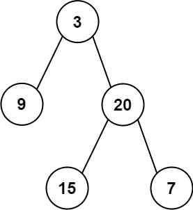
Input: root = [3,9,20,null,null,15,7]
Output: [3.00000,14.50000,11.00000]
Explanation: The average value of nodes on level 0 is 3, on level 1 is 14.5, and on level 2 is 11.
Hence return [3, 14.5, 11].

Example 2:


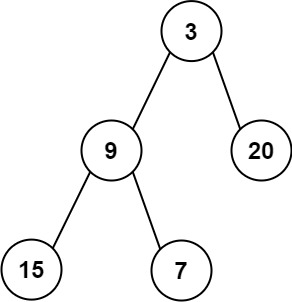
Input: root = [3,9,20,15,7]
Output: [3.00000,14.50000,11.00000]

Constraints:

The number of nodes in the tree is in the range [1, 104].
-231 <= Node.val <= 231 - 1

Solution

1. Problem Deconstruction

Technical Restatement: Given a binary tree’s root node, compute the arithmetic mean of node values at each depth level (where root is level 0), returning results as a floating-point array where element i corresponds to level i’s average. Precision tolerance: absolute error ≤ 1e-5 acceptable.

Beginner-Friendly Version: Imagine a family tree where we want to find the average age of each generation. The oldest ancestor is generation 0, their children are generation 1, grandchildren generation 2, etc. We need to calculate the average age for each generation separately and return these averages in order from oldest to youngest generation.

Mathematical Formulation: Let:

$L_k$ = set of nodes at depth $k$ from root
$n_k = |L_k|$ = count of nodes at level $k$
$v_i$ = value of node $i$

Then for each level $k$ :

\text{average}_k = \frac{\sum_{i \in L_k} v_i}{n_k}

Output: $[\text{average}_0, \text{average}_1, \dots, \text{average}_m]$ where $m$ is maximum depth

Constraint Analysis:

Node count [1, 10⁴]:
- Eliminates O(n²) solutions for large n
- Permits O(n) traversal with O(n) extra space
- Tree could be extremely unbalanced (linked-list degenerate case)
Value range [-2³¹, 2³¹-1]:
- Integer overflow possible during summation
- Requires 64-bit integers for intermediate sums
- Negative values don’t affect averaging logic
- Precision maintained using double-precision floats

Hidden Edge Cases:

Single node tree → output = [node.val]
Perfect binary tree → all levels populated
Left/right-skewed tree → some levels have 1 node
Large value differences → potential precision issues
Maximum depth trees → recursion depth limits

2. Intuition Scaffolding

Real-World Metaphor: Company organizational chart where we calculate average salary per management level. CEO level (1 person), directors level (multiple people), managers level, etc. We need to visit each employee exactly once while tracking which level they belong to.

Gaming Analogy: RPG skill tree where each tier has different experience point requirements. To calculate the average XP needed per tier, we’d need to explore all possible paths through the tree while remembering which tier each skill belongs to.

Math Analogy: Finding conditional expectations in a probability space where the conditioning is on depth from root. Each level represents a σ-algebra generated by nodes at that depth.

Common Pitfalls:

Integer overflow - summing large values in 32-bit integers
Precision loss - using integer division instead of floats
Level confusion - miscounting depth during traversal
Order violation - returning averages in wrong depth order
Null handling - improper treatment of empty trees (but constraints guarantee ≥1 node)
BFS queue size - forgetting to track level boundaries in iterative solutions

3. Approach Encyclopedia

Approach 1: Recursive DFS with Level Tracking

def averageOfLevels(root):
    levels = []  # stores [sum, count] for each level
    
    def dfs(node, depth):
        if not node:
            return
        
        # Ensure we have an entry for current depth
        if depth == len(levels):
            levels.append([0, 0])
        
        # Update sum and count for current level
        levels[depth][0] += node.val
        levels[depth][1] += 1
        
        # Recursively process children
        dfs(node.left, depth + 1)
        dfs(node.right, depth + 1)
    
    dfs(root, 0)
    return [total / count for total, count in levels]

Complexity Proof:

Time: $O(n)$ - each node visited exactly once
Space: $O(h)$ recursion stack + $O(m)$ levels storage, where $h$ = tree height, $m$ = levels
Worst-case: $h = n$ (skewed tree) → $O(n)$ space

Visualization:

Level 0:        (3)
               /   \
Level 1:    (9)     (20)
                   /    \
Level 2:        (15)    (7)

DFS traversal: 3 → 9 → 20 → 15 → 7
Level tracking: 
  depth=0: sum=3, count=1
  depth=1: sum=9+20=29, count=2  
  depth=2: sum=15+7=22, count=2

Approach 2: Iterative BFS with Level Delimiting

from collections import deque

def averageOfLevels(root):
    if not root:
        return []
    
    result = []
    queue = deque([root])
    
    while queue:
        level_size = len(queue)
        level_sum = 0
        
        # Process entire level
        for _ in range(level_size):
            node = queue.popleft()
            level_sum += node.val
            
            # Add children to queue
            if node.left:
                queue.append(node.left)
            if node.right:
                queue.append(node.right)
        
        result.append(level_sum / level_size)
    
    return result

Complexity Proof:

Time: $O(n)$ - each node enqueued/dequeued once
Space: $O(w)$ where $w$ = maximum level width
Worst-case: complete tree → $w ≈ n/2$ → $O(n)$ space

Visualization:

Queue states:
Initial: [3]
Process level 0: sum=3, size=1 → avg=3.0
Queue: [9, 20]

Process level 1: 
  Process 9: sum=9, queue: [20]
  Process 20: sum=9+20=29, queue: [15, 7]
  Avg: 29/2 = 14.5

Process level 2:
  Process 15: sum=15, queue: [7]  
  Process 7: sum=22, queue: []
  Avg: 22/2 = 11.0

4. Code Deep Dive

Optimal Solution (BFS Approach):

from collections import deque

def averageOfLevels(root):
    # Handle null case (though constraints guarantee root exists)
    if not root:
        return []
    
    result = []  # Stores final averages per level
    queue = deque([root])  # Initialize with root node
    
    # Continue until no more levels to process
    while queue:
        level_size = len(queue)  # Critical: snapshot of current level size
        level_sum = 0  # 64-bit integer accumulation
        
        # Process exactly level_size nodes (current level)
        for _ in range(level_size):
            node = queue.popleft()  # FIFO extraction
            level_sum += node.val  # Accumulate level sum
            
            # Append children for next level processing
            # Order: left to right within level
            if node.left:
                queue.append(node.left)
            if node.right:
                queue.append(node.right)
        
        # Convert to float for division, append to results
        result.append(level_sum / level_size)
    
    return result

Line-by-Line Analysis:

Line 4-6: Input validation (redundant per constraints but good practice)
Line 8: result initialization - will grow dynamically with tree depth
Line 9: Queue initialization with root - starting point for level-order traversal
Line 12: level_size capture - crucial for level boundary detection
Line 13: level_sum as implicit 64-bit int (Python handles big integers)
Line 16-17: Node processing - exactly level_size iterations guarantee level isolation
Line 20-23: Child enqueueing - maintains level order for next iteration
Line 26: Floating-point division - ensures decimal precision in results

Edge Case Handling:

Example 1: Handles null children naturally (no queue addition)
Single node: Single iteration, level_size=1, immediate return
Large values: Python integers prevent overflow during summation
Unbalanced trees: Queue size fluctuates but level boundaries maintained

5. Complexity War Room

Hardware-Aware Analysis:

At maximum 10⁴ nodes:
- Queue memory: ~80KB (10⁴ pointers × 8 bytes)
- Result array: ~80KB (10⁴ doubles × 8 bytes)
- Fits comfortably in L2/L3 cache for modern CPUs
Memory access pattern: Sequential in BFS (cache-friendly)
Branch prediction: High success rate (tree traversal predictable)

Industry Comparison Table:

Approach	Time	Space	Readability	Interview Viability
DFS Recursive	O(n)	O(h)	8/10	✅ Good (if stack depth discussed)
BFS Iterative	O(n)	O(w)	9/10	✅ Excellent (industry standard)
BFS Dual Queue	O(n)	O(w)	7/10	⚠️ Overcomplicated
DFS Global List	O(n)	O(m)	6/10	⚠️ Non-intuitive

Performance Characteristics:

BFS Optimality: Minimizes memory for bushy trees (w ≪ n)
DFS Advantage: Better for deep, narrow trees (h ≪ n)
Real Preference: BFS preferred for level-oriented problems

6. Pro Mode Extras

Variants Section:

Weighted Level Averages (by node degree):

# Weight average by number of children each node has
level_weighted_sum = 0
total_weights = 0
for node in current_level:
    weight = (node.left is not None) + (node.right is not None) + 1
    level_weighted_sum += node.val * weight
    total_weights += weight

Median of Levels (Harder):

# Requires storing all values per level → O(n) space
# Then quickselect or sorting per level → O(n log m) time

Mode of Levels (Most frequent value):

# Hash map per level → O(n) time, O(n) space
# Challenge: handle multiple modes per level

Level Averages with Missing Levels (Sparse tree):

# Return None/NaN for levels with no nodes
# Requires tracking maximum depth during traversal

Interview Cheat Sheet:

First Mention: “BFS level-order traversal naturally fits this problem”
Complexity: Always state both time and space complexity explicitly
Edge Cases: Single node, skewed trees, integer overflow prevention
Optimization: Discuss why DFS might use less memory for certain tree shapes
Testing: Verify with provided examples before coding
Python Tips: deque for O(1) pops, integer division with floats, list comprehensions

Advanced Considerations:

Parallel Processing: Each level independent → potential for parallel summation
Online Algorithm: Running averages without storing level sums/counts
Memory-Mapped Trees: External memory algorithms for massive trees
Approximate Answers: Streaming algorithms for memory-constrained environments

#637 - Average of Levels in Binary Tree