Spiral Matrix

Difficulty: Medium
Topics: Array, Matrix, Simulation
Link: https://leetcode.com/problems/spiral-matrix/

Problem Description

Given an m x n matrix, return all elements of the matrix in spiral order.

Example 1:


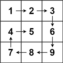
Input: matrix = [[1,2,3],[4,5,6],[7,8,9]]
Output: [1,2,3,6,9,8,7,4,5]

Example 2:


Input: matrix = [[1,2,3,4],[5,6,7,8],[9,10,11,12]]
Output: [1,2,3,4,8,12,11,10,9,5,6,7]

Constraints:

m == matrix.length
n == matrix[i].length
1 <= m, n <= 10
-100 <= matrix[i][j] <= 100

Solution

1. Problem Deconstruction

Technical Definition
Given an m × n matrix, traverse all elements in clockwise spiral order starting from the top-left corner. The traversal must:

Move right along the top row until the last column.
Move down along the right column until the last row.
Move left along the bottom row until the first column (if applicable).
Move up along the left column until the second row (if applicable).
Repeat steps 1–4 for the inner submatrix defined by updated boundaries, until all elements are visited.

Beginner Explanation
Imagine walking through a grid:

Start at the top-left corner, go right to the end.
Turn down, go to the bottom.
Turn left, go to the start of the row.
Turn up, stop just below the starting row.
Repeat this “right → down → left → up” pattern in the inner layers until every cell is covered.

Mathematical Formulation
Let M be an m × n matrix. Define boundaries:

t (top), b (bottom), l (left), r (right).
Initialize t = 0, b = m - 1, l = 0, r = n - 1. While t ≤ b and l ≤ r:

Right: Append M[t][j] for j = l to r.
Down: Append M[i][r] for i = t + 1 to b.
Left (if t < b): Append M[b][j] for j = r - 1 to l (reverse).
Up (if l < r): Append M[i][l] for i = b - 1 to t + 1 (reverse).
Update t++, b--, l++, r--. The sequence is the spiral order.

Constraint Analysis

1 ≤ m, n ≤ 10:
- Limits max elements to 100 → algorithms up to O(n⁴) are feasible, but O(mn) is optimal.
- Edge cases: Single row (m=1), single column (n=1), or single element (m=n=1).
-100 ≤ matrix[i][j] ≤ 100:
- Values fit in 32-bit integers → no overflow concerns.
Hidden edge cases:
- After traversing a layer, inner boundaries may collapse (e.g., t > b), requiring conditional checks to avoid duplication.

2. Intuition Scaffolding

Analogies

Real-World Metaphor: Peeling an onion layer-by-layer. The outer skin is removed first (perimeter), revealing smaller inner layers to peel similarly.
Gaming Analogy: A dungeon crawler moving right until hitting a wall, then turning clockwise to explore adjacent paths, marking visited cells.
Math Analogy: A space-filling curve (e.g., Hilbert curve variant) that linearly orders 2D grid points while preserving spatial locality.

Common Pitfalls

Duplication in single-row/column matrices:
- Traversing left/up after right/down without boundary checks repeats elements.
Ignoring boundary updates:
- Forgetting to shrink boundaries after a layer causes infinite loops.
Incorrect loop ranges:
- Using inclusive vs. exclusive bounds improperly skips or duplicates elements.
Over-reliance on visited markers:
- Using O(mn) space for tracking when boundary simulation suffices.
Misordering traversal directions:
- Swapping down/left or up/right breaks the spiral sequence.

3. Approach Encyclopedia

Approach 1: Boundary Simulation (Optimal)
Idea: Shrink layer boundaries after each clockwise traversal.
Pseudocode:

def spiralOrder(matrix):
    if not matrix: return []
    t, b = 0, len(matrix)-1
    l, r = 0, len(matrix[0])-1
    res = []
    while t <= b and l <= r:
        # Right
        for j in range(l, r+1):
            res.append(matrix[t][j])
        t += 1
        # Down
        for i in range(t, b+1):
            res.append(matrix[i][r])
        r -= 1
        # Left (if rows remain)
        if t <= b:
            for j in range(r, l-1, -1):
                res.append(matrix[b][j])
            b -= 1
        # Up (if columns remain)
        if l <= r:
            for i in range(b, t-1, -1):
                res.append(matrix[i][l])
            l += 1
    return res

Complexity Proof:

Time: Each element visited exactly once → Θ(mn).
Space: O(1) extra space (boundaries). Output is O(mn).

Visualization (3×3 Matrix):

Initial:       Step 1 (Right):   Step 2 (Down):    Step 3 (Left):   Step 4 (Up):
1 → 2 → 3      1 → 2 → 3        1 → 2 → 3         1 → 2 → 3         1 → 2 → 3
4    5    6          ↓               5               5 ← 6              5
7 ← 8 ← 9         4 → 5 → 6         ↓ ↓         Then Up: 4          Then Right: 5
                  Then Down: 9      7   8         (from 7)          (inner layer)

Approach 2: Visited Matrix
Idea: Track visited cells. Change direction upon boundary/visited hits.
Pseudocode:

def spiralOrder(matrix):
    if not matrix: return []
    m, n = len(matrix), len(matrix[0])
    visited = [[False]*n for _ in range(m)]
    dirs = [(0,1), (1,0), (0,-1), (-1,0)]  # Right, Down, Left, Up
    d = 0
    i, j = 0, 0
    res = []
    for _ in range(m*n):
        res.append(matrix[i][j])
        visited[i][j] = True
        ni, nj = i + dirs[d][0], j + dirs[d][1]
        if ni < 0 or ni >= m or nj < 0 or nj >= n or visited[ni][nj]:
            d = (d+1) % 4  # Turn clockwise
            ni, nj = i + dirs[d][0], j + dirs[d][1]
        i, j = ni, nj
    return res

Complexity:

Time: Θ(mn) (each cell processed once).
Space: Θ(mn) for visited matrix.

4. Code Deep Dive

Optimal Solution (Boundary Simulation)

def spiralOrder(matrix):
    if not matrix or not matrix[0]:  # Handle empty input
        return []
    t, b = 0, len(matrix)-1          # Top/bottom boundaries
    l, r = 0, len(matrix[0])-1       # Left/right boundaries
    res = []
    while t <= b and l <= r:          # Continue while layers exist
        # Right: Top row (l to r)
        for j in range(l, r+1):
            res.append(matrix[t][j])
        t += 1                       # Shrink top boundary
        
        # Down: Right column (t to b)
        for i in range(t, b+1):
            res.append(matrix[i][r])
        r -= 1                       # Shrink right boundary
        
        # Left: Bottom row (r to l, reverse) if rows remain
        if t <= b:                   # Avoid re-traversing single row
            for j in range(r, l-1, -1):
                res.append(matrix[b][j])
            b -= 1                   # Shrink bottom boundary
        
        # Up: Left column (b to t, reverse) if columns remain
        if l <= r:                   # Avoid re-traversing single column
            for i in range(b, t-1, -1):
                res.append(matrix[i][l])
            l += 1                   # Shrink left boundary
    return res

Edge Case Handling

Example 1 (3×3):
- Layer 1: Right (1,2,3) → Down (6,9) → Left (8,7) → Up (4) → Layer 2: Right (5).
Example 2 (3×4):
- Layer 1: Right (1,2,3,4) → Down (8,12) → Left (11,10,9) → Up (5) → Layer 2: Right (6,7).
Single Row (1×4):
- Right (1,2,3,4) → Down (none) → Left (skipped via t≤b) → Up (skipped via l≤r).
Single Column (4×1):
- Right (1) → Down (2,3,4) → Left (skipped) → Up (skipped).

5. Complexity War Room

Hardware-Aware Analysis

Max elements: 100 (10×10).
L1 Cache: ~64KB → 100 integers (400B) fits comfortably.
Memory: Boundaries use 4 integers (16B) → negligible.

Approach Comparison

Approach	Time	Space	Readability	Interview Viability
Boundary Simulation	`Θ(mn)`	`O(1)`	9/10	✅ Optimal
Visited Matrix	`Θ(mn)`	`Θ(mn)`	8/10	❌ (Wastes space)
Recursive Layers	`Θ(mn)`	`O(1)`	7/10	✅ (But iterative preferred)

6. Pro Mode Extras

Variants

Spiral Matrix II (LeetCode 59):
- Generate n×n matrix with elements 1 to n² in spiral order.
- Solution: Use boundary simulation to fill instead of traverse.
Counter-Clockwise Spiral:
- Traverse: Down → Right → Up → Left.
- Solution: Swap direction order and adjust boundaries.
Spiral Matrix III (LeetCode 885):
- Generate spiral coordinates starting from (r0, c0) expanding outward.
- Solution: Control steps (right 1, down 1, left 2, up 2, …) and expand.

Interview Cheat Sheet

Key Points:
1. Start with boundary initialization.
2. Explain direction order and boundary updates.
3. Emphasize checks for single-row/column cases.
Time/Space: Always state Θ(mn) time, O(1) space (excl. output).
Test Cases: Cover 1×1, 1×n, m×1, and rectangular matrices.

#54 - Spiral Matrix