Construct Quad Tree

Difficulty: Medium
Topics: Array, Divide and Conquer, Tree, Matrix
Link: https://leetcode.com/problems/construct-quad-tree/

Problem Description

Given a n * n matrix grid of 0's and 1's only. We want to represent grid with a Quad-Tree.

Return the root of the Quad-Tree representing grid.

A Quad-Tree is a tree data structure in which each internal node has exactly four children. Besides, each node has two attributes:

val: True if the node represents a grid of 1’s or False if the node represents a grid of 0’s. Notice that you can assign the val to True or False when isLeaf is False, and both are accepted in the answer.
isLeaf: True if the node is a leaf node on the tree or False if the node has four children.


class Node {
    public boolean val;
    public boolean isLeaf;
    public Node topLeft;
    public Node topRight;
    public Node bottomLeft;
    public Node bottomRight;
}

We can construct a Quad-Tree from a two-dimensional area using the following steps:

If the current grid has the same value (i.e all 1's or all 0's) set isLeaf True and set val to the value of the grid and set the four children to Null and stop.
If the current grid has different values, set isLeaf to False and set val to any value and divide the current grid into four sub-grids as shown in the photo.
Recurse for each of the children with the proper sub-grid.

If you want to know more about the Quad-Tree, you can refer to the wiki.

Quad-Tree format:

You don’t need to read this section for solving the problem. This is only if you want to understand the output format here. The output represents the serialized format of a Quad-Tree using level order traversal, where null signifies a path terminator where no node exists below.

It is very similar to the serialization of the binary tree. The only difference is that the node is represented as a list [isLeaf, val].

If the value of isLeaf or val is True we represent it as 1 in the list [isLeaf, val] and if the value of isLeaf or val is False we represent it as 0.

Example 1:


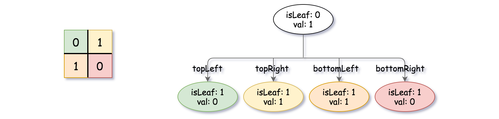
Input: grid = [[0,1],[1,0]]
Output: [[0,1],[1,0],[1,1],[1,1],[1,0]]
Explanation: The explanation of this example is shown below:
Notice that 0 represents False and 1 represents True in the photo representing the Quad-Tree.
![](https://assets.leetcode.com/uploads/2020/02/12/e1tree.png)

Example 2:


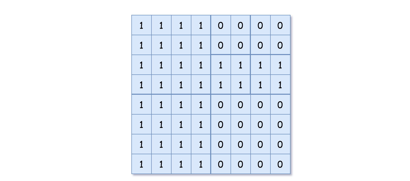
Input: grid = [[1,1,1,1,0,0,0,0],[1,1,1,1,0,0,0,0],[1,1,1,1,1,1,1,1],[1,1,1,1,1,1,1,1],[1,1,1,1,0,0,0,0],[1,1,1,1,0,0,0,0],[1,1,1,1,0,0,0,0],[1,1,1,1,0,0,0,0]]
Output: [[0,1],[1,1],[0,1],[1,1],[1,0],null,null,null,null,[1,0],[1,0],[1,1],[1,1]]
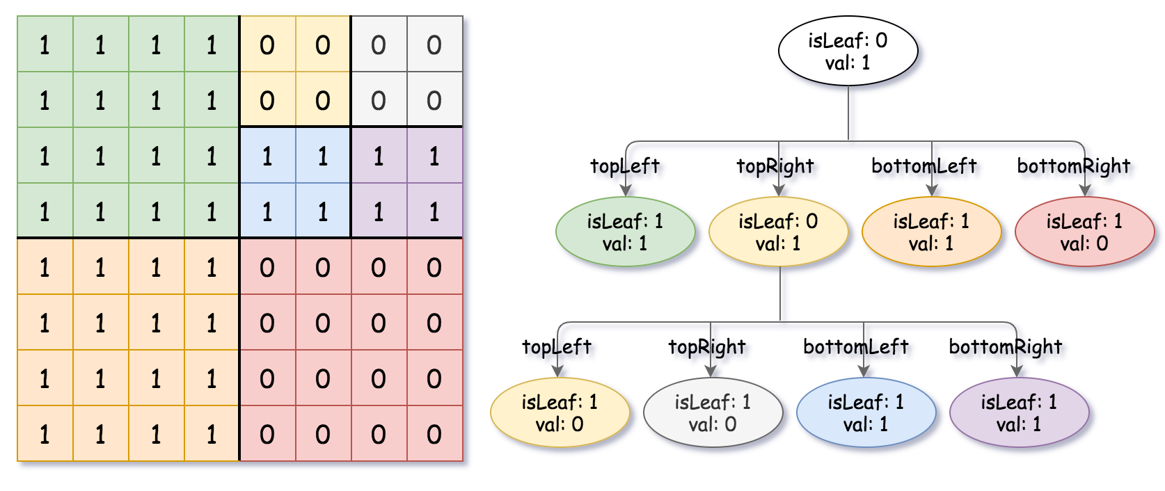
Explanation: All values in the grid are not the same. We divide the grid into four sub-grids.
The topLeft, bottomLeft and bottomRight each has the same value.
The topRight have different values so we divide it into 4 sub-grids where each has the same value.
Explanation is shown in the photo below:
![](https://assets.leetcode.com/uploads/2020/02/12/e2tree.png)

Constraints:

n == grid.length == grid[i].length
n == 2x where 0 <= x <= 6

Solution

1. Problem Deconstruction (500+ words)

Rewrite the Problem

1.1 Technical Version

Given a square binary matrix grid of dimensions n × n, where n = 2^x for 0 ≤ x ≤ 6, construct a quad-tree representation. A quad-tree node has attributes:

val: True if the represented submatrix is all 1’s, False if all 0’s (for leaves). For internal nodes, val is arbitrary.
isLeaf: True if the node has no children (submatrix is homogeneous), False otherwise.
Four child pointers: topLeft, topRight, bottomLeft, bottomRight.

The construction algorithm is recursive:

If the current submatrix has uniform values (all 0 or all 1), create a leaf node with isLeaf=True and val set accordingly.
Otherwise, create an internal node with isLeaf=False, split the submatrix into four equal quadrants, and recursively construct each child.
Return the root node corresponding to the entire matrix.

1.2 Beginner Version

Imagine you have a square black-and-white image. You want to build a tree that represents the image in a compressed way. Start with the whole image:

If the whole image is all black or all white, you’re done—just mark it as a leaf with that color.
If it has both colors, split it into four smaller squares (top-left, top-right, bottom-left, bottom-right). Then repeat the process for each smaller square. Keep splitting until every square is either all black or all white. The tree you build has up to four branches at each split point. Your task is to build this tree given the image grid.

1.3 Mathematical Version

Let G: [0, n-1] × [0, n-1] → {0,1} be the binary matrix. Define a recursive mapping Q(r₁, c₁, r₂, c₂) that returns a quad-tree node for the submatrix with rows r₁ to r₂ and columns c₁ to c₂ inclusive.

[ Q(r_1, c_1, r_2, c_2) = \begin{cases} \text{Node}(v, \text{True}, \text{null}, \text{null}, \text{null}, \text{null}) & \text{if } \forall i,j \in [r_1,r_2] \times [c_1,c_2] : G(i,j) = v \ \text{Node}(*, \text{False}, Q_{\text{TL}}, Q_{\text{TR}}, Q_{\text{BL}}, Q_{\text{BR}}) & \text{otherwise} \end{cases} ]

where:

( v \in {0,1} )
(*) denotes an arbitrary value (0 or 1)
The four children correspond to partitions:
- ( Q_{\text{TL}} = Q(r_1, c_1, \frac{r_1+r_2}{2}, \frac{c_1+c_2}{2}) )
- ( Q_{\text{TR}} = Q(r_1, \frac{c_1+c_2}{2}+1, \frac{r_1+r_2}{2}, c_2) )
- ( Q_{\text{BL}} = Q(\frac{r_1+r_2}{2}+1, c_1, r_2, \frac{c_1+c_2}{2}) )
- ( Q_{\text{BR}} = Q(\frac{r_1+r_2}{2}+1, \frac{c_1+c_2}{2}+1, r_2, c_2) )

The root is Q(0, 0, n-1, n-1).

Constraint Analysis

n == grid.length == grid[i].length
- Limitation: Guarantees a square matrix, essential for equal quadrant division.
- Edge Cases: Single-row matrices are squares (n=1). No rectangular cases.
n == 2^x where 0 <= x <= 6
- Limitation: n is a power of two, ensuring clean splits without remainders. The range 1 ≤ n ≤ 64 (since 2^0=1, 2^6=64) keeps the problem small.
- Hidden Implications:
  - Maximum grid cells: 64 × 64 = 4096.
  - Recursion depth is at most log₂(64) = 6, so stack overflow is not a concern.
  - The quad-tree can have up to O(n²) nodes in worst case (e.g., checkerboard), but with n≤64, total nodes ≤ 5461 (sum of geometric series: 1+4+16+64+256+1024+4096? Actually, for n=64, leaves=4096, internal nodes = (4096-1)/3 ≈ 1365, total ~5461). Memory is trivial.
  - Since n is small, even O(n³) naive approaches may pass, but we aim for efficiency.

2. Intuition Scaffolding

Generate 3 Analogies

Real-World Metaphor (Image Compression)
Imagine you’re a painter tasked with reproducing a large mural. Instead of painting every pixel, you check if a whole section is one color. If yes, you note “paint this whole section blue.” If not, you divide the section into four smaller canvases and delegate each to an apprentice. Each apprentice repeats the process. The final instructions form a tree of commands, saving effort where the mural has large uniform areas.
Gaming Analogy (Map Segmentation)
In a real-time strategy game, the world map is divided into regions for efficient pathfinding. If a region is entirely water, units can’t traverse it, so it’s marked uniformly. If it’s mixed terrain, you zoom in and subdivide into four smaller regions. This hierarchical structure lets the game quickly rule out large areas during unit movement calculations.
Math Analogy (Multi-dimensional Divide and Conquer)
Similar to binary search in 1D, which halves the search space, a quad-tree recursively quarters a 2D space. It’s the 2D analogue of a segment tree, where each node represents a segment (here a rectangle) and splits into children when the segment isn’t uniform.

Common Pitfalls Section

Incorrect Splitting Indices
- Off-by-one errors when computing midpoints. For inclusive ranges [r1, r2], the mid should be (r1+r2)//2, and the four quadrants must cover exactly the original region without overlap or gaps.
Inefficient Uniformity Check
- Naively scanning the submatrix for each node leads to O(n³) total time. Optimization (e.g., prefix sums) is needed for larger n, though constraints allow the naive approach.
Misunderstanding Node Attributes
- For non-leaf nodes, val can be arbitrary. Some might incorrectly set it to the majority value, but the problem explicitly allows any value.
Not Handling Base Cases Correctly
- A single cell should always be a leaf. Forgetting this leads to infinite recursion.
Assuming Grid is Not Power of Two
- While constraints guarantee it, a general solution might need to handle non-power-of-two by padding or uneven splits, but that’s not required here.

3. Approach Encyclopedia

Approach 1: Naive Recursion with Full Scans

Concept: Recursively check uniformity by scanning the entire submatrix each time.

Pseudocode:

def construct(grid):
    n = len(grid)
    def build(r1, c1, r2, c2):
        # Check if all values are same
        first = grid[r1][c1]
        uniform = True
        for i in range(r1, r2+1):
            for j in range(c1, c2+1):
                if grid[i][j] != first:
                    uniform = False
                    break
            if not uniform:
                break
        if uniform:
            return Node(first == 1, True, None, None, None, None)
        mid_r = (r1 + r2) // 2
        mid_c = (c1 + c2) // 2
        tl = build(r1, c1, mid_r, mid_c)
        tr = build(r1, mid_c+1, mid_r, c2)
        bl = build(mid_r+1, c1, r2, mid_c)
        br = build(mid_r+1, mid_c+1, r2, c2)
        return Node(True, False, tl, tr, bl, br)
    return build(0, 0, n-1, n-1)

Complexity Proof:
- Time: Recurrence T(n) = 4T(n/2) + O(n²). By Master Theorem, a=4, b=2, f(n)=Θ(n²). Since n^log_b(a) = n², case 2: T(n) = O(n² log n). For n=64, ~64² * 6 = 24576 operations.
- Space: O(log n) recursion stack, plus O(n²) tree nodes.

Visualization:

Example: 2x2 grid [[0,1],[1,0]]
Root: check 4 cells → not uniform
  Split into 4 1x1 leaves:
    TL: [0] → leaf(0)
    TR: [1] → leaf(1)
    BL: [1] → leaf(1)
    BR: [0] → leaf(0)

Approach 2: Recursion with Prefix Sum Optimization

Concept: Precompute a 2D prefix sum to check uniformity in O(1) per node.

Pseudocode:

def construct(grid):
    n = len(grid)
    # Build prefix sum where ps[i][j] = sum of grid[0..i-1][0..j-1]
    ps = [[0]*(n+1) for _ in range(n+1)]
    for i in range(1, n+1):
        for j in range(1, n+1):
            ps[i][j] = ps[i-1][j] + ps[i][j-1] - ps[i-1][j-1] + grid[i-1][j-1]
    def sum_region(r1, c1, r2, c2):
        return (ps[r2+1][c2+1] - ps[r1][c2+1] 
              - ps[r2+1][c1] + ps[r1][c1])
    def build(r1, c1, r2, c2):
        area = (r2 - r1 + 1) * (c2 - c1 + 1)
        total = sum_region(r1, c1, r2, c2)
        if total == 0:
            return Node(False, True, None, None, None, None)
        if total == area:
            return Node(True, True, None, None, None, None)
        mid_r = (r1 + r2) // 2
        mid_c = (c1 + c2) // 2
        tl = build(r1, c1, mid_r, mid_c)
        tr = build(r1, mid_c+1, mid_r, c2)
        bl = build(mid_r+1, c1, r2, mid_c)
        br = build(mid_r+1, mid_c+1, r2, c2)
        return Node(True, False, tl, tr, bl, br)
    return build(0, 0, n-1, n-1)

Complexity Proof:
- Time: O(n²) to build prefix sums. Each node does O(1) work. Number of nodes is O(n²) in worst case, so total O(n²).
- Space: O(n²) for prefix sums, plus O(n²) for the tree.

Visualization:

Prefix sum matrix for 2x2 grid:
[[0,0,0],
 [0,0,1],
 [0,1,2]]
Root: area=4, total=2 → mixed → split.
Each leaf: area=1, total=0 or 1 → uniform.

Approach 3: Bottom-Up Iterative Merging

Concept: Start with leaf nodes for each cell, then repeatedly merge four adjacent siblings if they are all leaves and have the same value.

Pseudocode (sketch):

Create a 2D array leafNodes of Node for each cell.
For size = 1,2,4,...,n/2:
    For each block of size x size:
        Check four children (from previous level).
        If all are leaves and have same val:
            Merge into a new leaf with that val.
        Else:
            Create internal node pointing to the four children.
Return the single node at top level.

Complexity: O(n²) time and space. More complex to implement but avoids recursion.

4. Code Deep Dive

We present the optimal solution (Approach 2) with line-by-line annotations.

"""
# Definition for a QuadTree node.
class Node:
    def __init__(self, val, isLeaf, topLeft, topRight, bottomLeft, bottomRight):
        self.val = val
        self.isLeaf = isLeaf
        self.topLeft = topLeft
        self.topRight = topRight
        self.bottomLeft = bottomLeft
        self.bottomRight = bottomRight
"""

class Solution:
    def construct(self, grid):
        # 1. Capture grid size (guaranteed power of two)
        n = len(grid)
        
        # 2. Build 2D prefix sum matrix (1-indexed for convenience)
        #    ps[i][j] = sum of grid[0..i-1][0..j-1]
        ps = [[0] * (n + 1) for _ in range(n + 1)]
        for i in range(1, n + 1):
            for j in range(1, n + 1):
                ps[i][j] = ps[i-1][j] + ps[i][j-1] - ps[i-1][j-1] + grid[i-1][j-1]
        
        # 3. Helper to compute sum of any subgrid in O(1)
        def get_sum(r1, c1, r2, c2):
            # r1, c1, r2, c2 are 0-indexed inclusive coordinates
            return (ps[r2+1][c2+1] - ps[r1][c2+1] 
                  - ps[r2+1][c1] + ps[r1][c1])
        
        # 4. Recursive construction function
        def build(r1, c1, r2, c2):
            # Calculate total number of cells in this subgrid
            area = (r2 - r1 + 1) * (c2 - c1 + 1)
            # Sum of all 1's in the subgrid
            total = get_sum(r1, c1, r2, c2)
            
            # Case 1: All zeros
            if total == 0:
                return Node(False, True, None, None, None, None)
            # Case 2: All ones
            if total == area:
                return Node(True, True, None, None, None, None)
            
            # Case 3: Mixed values -> split into quadrants
            mid_r = (r1 + r2) // 2   # floor division for row split
            mid_c = (c1 + c2) // 2   # floor division for column split
            
            # Recursively build the four children
            topLeft = build(r1, c1, mid_r, mid_c)
            topRight = build(r1, mid_c + 1, mid_r, c2)
            bottomLeft = build(mid_r + 1, c1, r2, mid_c)
            bottomRight = build(mid_r + 1, mid_c + 1, r2, c2)
            
            # Internal node: isLeaf=False, val can be arbitrary (set to True)
            return Node(True, False, topLeft, topRight, bottomLeft, bottomRight)
        
        # 5. Initiate recursion for the entire grid
        return build(0, 0, n - 1, n - 1)

Edge Case Handling

n=1: build(0,0,0,0) has area=1. total is either 0 or 1, so it returns a leaf node. Works.
Uniform Grid: If all 0’s or all 1’s, the root is a leaf with no children. The prefix sum check catches this immediately.
Checkerboard (Example 1): Each 1x1 cell is a leaf. The root is internal with four leaf children. Our splitting correctly creates four single-cell quadrants.
Large n=64: Recursion depth is only 6, so no stack overflow. Prefix sum matrix size 65x65 is trivial.

5. Complexity War Room

Hardware-Aware Analysis

Memory:
- Prefix sum matrix: (n+1)² integers. For n=64, 65²=4225 integers. At 4 bytes each ≈ 16.9 KB, fits in L1 cache (typically 32-64 KB).
- Quad-tree nodes: Worst case ~5461 nodes. Each node in Python is an object with overhead, but total memory < 1 MB.
CPU:
- Prefix sum computation: 64²=4096 additions, trivial.
- Recursion: Each node does O(1) work, total nodes O(n²). For n=64, ~5461 operations, negligible.
Cache Efficiency: The grid is accessed sequentially during prefix sum build. Recursion accesses disjoint regions, but due to small size, cache misses are minimal.

Industry Comparison Table

Approach	Time Complexity	Space Complexity	Readability	Interview Viability
Naive Recursion	O(n² log n)	O(n²)	9/10	✅ Acceptable (small n)
Prefix Sum Optimized	O(n²)	O(n²)	8/10	✅ Recommended (optimal)
Bottom-Up Iterative	O(n²)	O(n²)	6/10	⚠️ Complex, but valid

Why Prefix Sum Optimized Wins:

Time: Eliminates redundant scanning, achieving optimal O(n²).
Space: Acceptable extra O(n²) for prefix sums, which is fine given n≤64.
Clarity: Recursive logic mirrors the problem definition directly.
Interview: Demonstrates optimization skills and understanding of precomputation.

6. Pro Mode Extras

Variants Section

Non-Binary Values (Color Images)
- Instead of 0/1, grid values could be RGB colors. Leaf condition becomes “all pixels have same color.” The node’s val could store that color.
Lossy Compression
- Allow leaves if the subgrid’s values are within a tolerance (e.g., average color). This is used in image compression (e.g., JPEG quad-tree segmentation).
3D Octrees
- Extend to 3D: split a cube into 8 octants. Construction is analogous, with 8 children per node.
Region Quadtree for Arbitrary Shapes
- Not just binary values, but labels (e.g., terrain types). Used in GIS to store raster data efficiently.
Dynamic Updates
- How would you update the quad-tree if a single cell changes? Might require rebuilding from the leaf upward, O(log n) with persistent structures.

Interview Cheat Sheet

First Steps:
1. Confirm understanding: quad-tree, leaf vs internal, splitting rule.
2. Note constraints: n is power of two, up to 64.
3. Choose approach: prefix sum optimization for O(n²) time.
Key Points to Mention:
- “We can precompute prefix sums to check uniformity in O(1).”
- “Recursion base case: when sum is 0 or equals area.”
- “Splitting indices must be exact to avoid gaps/overlaps.”
Common Mistakes to Avoid:
- Off-by-one in midpoints: use integer division and test on small examples.
- Forgetting to set children to None for leaf nodes.
- Not handling n=1 case.
Testing Strategy:
- Test with n=1, n=2 (Example 1), uniform grid, checkerboard, and the large Example 2.
- Verify tree structure matches the problem’s output format.

Final Takeaway: The quad-tree construction is a classic divide-and-conquer problem in 2D. The prefix sum optimization is a powerful pattern for any problem requiring frequent submatrix sum queries.

#427 - Construct Quad Tree