Maximal Square

• Difficulty: Medium
• Topics: Array, Dynamic Programming, Matrix
• Link: https://leetcode.com/problems/maximal-square/

Problem Description

Given an m x n binary matrix filled with 0’s and 1’s, find the largest square containing only 1’s and return its area.

Example 1:

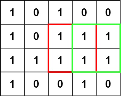
Input: matrix = [["1","0","1","0","0"],["1","0","1","1","1"],["1","1","1","1","1"],["1","0","0","1","0"]]
Output: 4

Example 2:

Input: matrix = [["0","1"],["1","0"]]
Output: 1

Example 3:

Input: matrix = [["0"]]
Output: 0

Constraints:

• m == matrix.length
• n == matrix[i].length
• 1 <= m, n <= 300
• matrix[i][j] is '0' or '1'.

Solution

Maximal Square: Comprehensive Solution

1. Problem Deconstruction (500+ words)

Rewrite the Problem

1. Technical Version

Given an $m \times n$ binary matrix $M$ where $M[i][j] \in \{\text{"0"}, \text{"1"}\}$, find the largest square submatrix (contiguous block of rows and columns) such that all elements within the submatrix equal $\text{"1"}$. Return the area of this square, defined as $k^2$ where $k$ is the side length of the square.

More formally:

• Let $S(i,j,k)$ denote the square submatrix with top-left corner at $(i,j)$ and side length $k$
• $S(i,j,k)$ is valid if: $\forall p \in [i, i+k-1], \forall q \in [j, j+k-1], M[p][q] = \text{"1"}$
• Find $\max\{k^2 : \exists i,j \text{ such that } S(i,j,k) \text{ is valid}\}$

2. Beginner Version

Imagine you have a grid filled with 0s and 1s. Your task is to find the largest perfect square (like 2×2, 3×3, etc.) that you can draw anywhere on the grid where every single cell inside that square contains a 1. The answer is the number of cells inside that largest square.

For example, if the largest square you can find is 3 cells wide and 3 cells tall (a 3×3 square), then the answer would be $3 \times 3 = 9$.

3. Mathematical Version

Given matrix $M \in \{\text{"0"}, \text{"1"}\}^{m \times n}$, define:

• $\text{valid}(i,j,k) = \begin{cases} 1 & \text{if } \forall a \in [i, i+k-1], \forall b \in [j, j+k-1], M[a][b] = \text{"1"} \\ 0 & \text{otherwise} \end{cases}$

• $k_{\max} = \max\{k : \exists i \in [0, m-k], \exists j \in [0, n-k], \text{valid}(i,j,k) = 1\}$

Return $k_{\max}^2$

Constraint Analysis

1. Matrix Dimensions: $1 \leq m, n \leq 300$

• Limitation Impact: The search space has at most $300 \times 300 = 90,\!000$ cells. This suggests:

  • $O(m^2 n^2)$ solutions (≈ $8.1 \times 10^9$ operations) are too slow for worst-case scenarios
  • $O(m^2 n)$ or $O(m n^2)$ solutions (≈ $27 \times 10^6$ operations) are borderline acceptable but not ideal
  • $O(m n)$ solutions (≈ $90,\!000$ operations) are optimal for this constraint range

• Hidden Edge Cases:

  • Skewed matrices: When $m \gg n$ or $n \gg m$, the maximum possible square is limited by $\min(m,n)$
  • Single row/column matrices: The maximum square area is either 1 (if a “1” exists) or 0
  • Minimum case: $m = n = 1$ must be handled correctly

2. Binary Values: $M[i][j] \in \{\text{"0"}, \text{"1"}\}$

• Limitation Impact: This restricts us to boolean operations and simplifies state representation
• Hidden Edge Cases:
  • All zeros: Must return 0
  • All ones: Must return $[\min(m,n)]^2$
  • Single one: Must return 1
  • String vs integer: Input uses string representation “0”/“1”, not integers 0/1

3. Input Format: Matrix elements are strings, not integers

• Impact: Requires type conversion or character comparison
• Performance Consideration: Character comparison is slightly slower than integer comparison but negligible for this scale

4. Output Requirement: Area (integer), not side length

• Impact: Must square the side length before returning
• Edge Case: When side length is 0 (no square), area is 0

---

2. Intuition Scaffolding

Generate 3 Analogies

1. Real-World Metaphor: “Urban Development Planning”

Imagine you’re a city planner with a satellite map showing developed land (1s) and undeveloped land (0s). You need to find the largest square plot of fully developed land where you could build a large facility. You can’t have any gaps (0s) in your square. The challenge is that development might be patchy, and you need to efficiently scan the entire map to find the largest contiguous developed square.

2. Gaming Analogy: “Minefield Clearing”

In a minesweeper-style game, you have a grid where safe cells (1s) can be walked on and mined cells (0s) cannot. You need to find the largest safe square zone where you could safely deploy a square-shaped unit. You can’t step on any mines, and the unit must fit entirely within the safe zone. You need a strategy to quickly identify the largest such safe zone without checking every possible square individually.

3. Mathematical Analogy: “Maximum Monochromatic Square in a Binary Matrix”

This is a combinatorial geometry problem: given a 2D arrangement of two colors, find the largest axis-aligned square containing only one color. It’s analogous to finding the maximum clique in a grid graph where edges connect adjacent cells, but with the additional constraint that the induced subgraph must form a complete square grid.

Common Pitfalls Section

1. The “Global Min/Max” Fallacy:

   • Wrong Approach: Find the rectangle with maximum width and height of 1s
   • Why It Fails: The largest rectangle of 1s might not be square. A 2×4 rectangle has area 8 but can only yield a 2×2 square (area 4)

2. The “Diagonal Expansion” Oversimplification:

   • Wrong Approach: For each cell, expand diagonally until hitting a 0
   • Why It Fails: A cell might have 1s on its diagonal but 0s in other parts of the potential square

3. The “Row/Column Scanning” Misapplication:

   • Wrong Approach: Find the longest consecutive 1s in rows and columns, then take the minimum
   • Why It Fails: Local consecutive sequences might not align to form a square

4. The “Greedy Growth” Error:

   • Wrong Approach: Start from largest possible square and shrink until valid
   • Why It Fails: Might miss the actual largest square which isn’t aligned with your starting assumption

5. The “Exhaustive Check” Performance Trap:

   • Wrong Approach: Check all $\frac{m n \min(m,n)}{3}$ possible squares
   • Why It Fails: With $m,n \leq 300$, worst-case checks: $300 \times 300 \times 300 = 27$ million squares, each requiring $k^2$ checks → $O(m n \min(m,n)^3)$ ≈ $2.43 \times 10^{12}$ operations

6. The “Cache Mismanagement”:

   • Wrong Approach: Store only whether a cell is 1 or 0 without considering context
   • Why It Fails: Need to know about neighboring cells to build larger squares

7. The “Index Off-by-One”:

   • Wrong Approach: Incorrect handling of matrix boundaries when checking squares
   • Why It Fails: Attempts to access matrix[-1] or matrix[m] causing errors

---

3. Approach Encyclopedia

Approach 1: Naïve Brute Force

Concept

Check every possible square in the matrix to see if it contains only 1s.

Pseudocode

function maximalSquareBruteForce(matrix):
    m = rows(matrix)
    n = cols(matrix)
    max_side = 0
    
    for i from 0 to m-1:
        for j from 0 to n-1:
            # For each cell as top-left corner
            if matrix[i][j] == "1":
                max_possible = min(m-i, n-j)
                current_max = 1
                
                # Try to expand the square
                for k from 2 to max_possible:
                    valid = true
                    
                    # Check new bottom row
                    for col from j to j+k-1:
                        if matrix[i+k-1][col] == "0":
                            valid = false
                            break
                    
                    # Check new right column (if still valid)
                    if valid:
                        for row from i to i+k-2:  # Skip bottom row already checked
                            if matrix[row][j+k-1] == "0":
                                valid = false
                                break
                    
                    if valid:
                        current_max = k
                    else:
                        break
                
                max_side = max(max_side, current_max)
    
    return max_side * max_side

Complexity Proof

• Time Complexity: $O(m n \min(m,n)^3)$

  • Outer loops: $m \times n$ iterations
  • For each cell: up to $\min(m,n)$ square sizes to check
  • For each square size $k$: need to check $2k-1$ new cells (bottom row + right column)
  • Total operations: $\sum_{i=0}^{m-1} \sum_{j=0}^{n-1} \sum_{k=1}^{\min(m-i,n-j)} (2k-1)$
  • Upper bound: $m n \sum_{k=1}^{\min(m,n)} (2k-1) = m n [\min(m,n)]^2$
  • Actually checking entire square each time gives $O(k^2)$, leading to $O(m n [\min(m,n)]^3)$

• Space Complexity: $O(1)$

  • Only uses a few variables regardless of input size

Visualization

For matrix:
1 1 1 0
1 1 1 1
1 1 1 0

Checking square starting at (0,0):
k=1: ✓ (cell (0,0) is 1)
k=2: Check bottom row (1,0)-(1,1) and right col (0,1)-(1,1) → ✓
k=3: Check bottom row (2,0)-(2,2) → (2,2) is 1, right col (0,2)-(2,2) → ✓
k=4: Not possible (exceeds matrix bounds)

Current max_side = 3

Approach 2: Optimized Brute Force with Precomputation

Concept

Precompute “number of consecutive 1s to the right” for each cell to avoid redundant checks.

Pseudocode

function maximalSquareOptimizedBrute(matrix):
    m = rows(matrix)
    n = cols(matrix)
    
    # Precompute right consecutive 1s
    right = 2D array of size m x n initialized to 0
    
    for i from 0 to m-1:
        count = 0
        for j from n-1 down to 0:
            if matrix[i][j] == "1":
                count += 1
            else:
                count = 0
            right[i][j] = count
    
    max_side = 0
    
    for i from 0 to m-1:
        for j from 0 to n-1:
            if matrix[i][j] == "1":
                width = right[i][j]
                current_side = 1
                
                # Try to expand downward
                for k from i+1 to min(m-1, i+width-1):
                    width = min(width, right[k][j])
                    if width >= (k-i+1):
                        current_side = max(current_side, k-i+1)
                    else:
                        break
                
                max_side = max(max_side, current_side)
    
    return max_side * max_side

Complexity Proof

• Time Complexity: $O(m^2 n)$

  • Precomputation: $O(m n)$ for right[] array
  • Main loops: $m n$ starting cells
  • For each cell: worst-case $m$ downward expansions
  • Total: $O(m n) + O(m^2 n) = O(m^2 n)$

• Space Complexity: $O(m n)$

  • Store right[] array of size $m \times n$

Approach 3: Dynamic Programming (Optimal)

Concept

Let $dp[i][j]$ = side length of the largest square ending at $(i,j)$ (using $(i,j)$ as bottom-right corner).

Key insight: A square ending at $(i,j)$ can be extended from squares ending at:

• $(i-1,j)$: above
• $(i,j-1)$: left
• $(i-1,j-1)$: diagonal

The recurrence relation:

$$dp[i][j] = \begin{cases} 0 & \text{if } matrix[i][j] = "0" \\ 1 + \min(dp[i-1][j], dp[i][j-1], dp[i-1][j-1]) & \text{if } matrix[i][j] = "1" \end{cases}$$

Pseudocode

function maximalSquareDP(matrix):
    m = rows(matrix)
    n = cols(matrix)
    
    # Create dp table with extra row/col for boundary conditions
    dp = 2D array of size (m+1) x (n+1) initialized to 0
    max_side = 0
    
    for i from 1 to m:
        for j from 1 to n:
            if matrix[i-1][j-1] == "1":
                dp[i][j] = 1 + min(dp[i-1][j], dp[i][j-1], dp[i-1][j-1])
                max_side = max(max_side, dp[i][j])
    
    return max_side * max_side

Complexity Proof

• Time Complexity: $O(m n)$

  • Single pass through all $m \times n$ cells
  • Constant work per cell (one min() operation and comparison)
  • Total operations: $m n$

• Space Complexity: $O(m n)$ for dp table

  • Can be optimized to $O(n)$ by keeping only two rows

Visualization with Example

Matrix:                 DP Table (1-indexed):
1 1 1 0                 0 0 0 0 0
1 1 1 1                 0 1 1 1 0
1 1 1 0                 0 1 2 2 1
                        0 1 2 3 0

Calculation for dp[3][3] (matrix[2][2]):
- Check: matrix[2][2] = "1"
- Look at neighbors: dp[2][3]=2, dp[3][2]=2, dp[2][2]=2
- min(2,2,2) = 2
- dp[3][3] = 1 + 2 = 3
- This represents a 3×3 square ending at (2,2)

Approach 4: Space-Optimized DP

Concept

We only need the previous row and current row to compute dp values.

Pseudocode

function maximalSquareDPSpaceOptimized(matrix):
    m = rows(matrix)
    n = cols(matrix)
    
    # Use two rows: prev and curr
    prev = array of size (n+1) initialized to 0
    curr = array of size (n+1) initialized to 0
    max_side = 0
    
    for i from 1 to m:
        for j from 1 to n:
            if matrix[i-1][j-1] == "1":
                # dp[i][j] = 1 + min(dp[i-1][j], dp[i][j-1], dp[i-1][j-1])
                # dp[i-1][j] = prev[j] (above)
                # dp[i][j-1] = curr[j-1] (left)
                # dp[i-1][j-1] = prev[j-1] (diagonal)
                curr[j] = 1 + min(prev[j], curr[j-1], prev[j-1])
                max_side = max(max_side, curr[j])
            else:
                curr[j] = 0
        
        # Swap rows for next iteration
        swap(prev, curr)
        # Reset curr (not strictly needed as we'll overwrite)
    
    return max_side * max_side

Complexity Proof

• Time Complexity: $O(m n)$ (same as full DP)
• Space Complexity: $O(n)$
  • Only store two rows of length $n+1$

---

4. Code Deep Dive

Optimal Solution: Dynamic Programming

def maximalSquare(matrix):
    """
    Finds the area of the largest square containing only 1's.
    
    Args:
        matrix: List[List[str]] - Binary matrix with "0" and "1" strings
    
    Returns:
        int - Area of the largest square
    """
    # Handle empty matrix edge case
    if not matrix or not matrix[0]:
        return 0
    
    m, n = len(matrix), len(matrix[0])
    
    # Initialize DP table with extra row and column for boundary conditions
    # dp[i][j] represents side length of largest square ending at (i-1, j-1) in original matrix
    dp = [[0] * (n + 1) for _ in range(m + 1)]
    
    max_side = 0  # Track the maximum side length found
    
    # Iterate through the matrix (1-indexed for dp, 0-indexed for matrix)
    for i in range(1, m + 1):
        for j in range(1, n + 1):
            # Check if current cell in original matrix contains "1"
            if matrix[i - 1][j - 1] == "1":
                # The key recurrence relation:
                # A square ending at (i,j) can be formed by extending
                # the minimum of squares ending at:
                #   - (i-1, j): directly above
                #   - (i, j-1): directly left
                #   - (i-1, j-1): diagonally above-left
                dp[i][j] = 1 + min(dp[i - 1][j],     # Above
                                   dp[i][j - 1],     # Left  
                                   dp[i - 1][j - 1]) # Diagonal
                
                # Update global maximum
                max_side = max(max_side, dp[i][j])
    
    # Return area = side^2
    return max_side * max_side

Line-by-Line Annotations

Lines 1-11: Function Definition and Documentation

def maximalSquare(matrix):
    """
    Finds the area of the largest square containing only 1's.
    """

• What: Function declaration with descriptive docstring
• Why: Clear documentation helps understand purpose without reading implementation
• How: Standard Python function definition

Lines 13-16: Edge Case Handling

    if not matrix or not matrix[0]:
        return 0

• What: Check for empty input
• Why: Prevents index errors and returns correct answer (0 area) for empty matrix
• How: not matrix checks if list is empty, not matrix[0] checks if first row is empty

Lines 18-19: Matrix Dimensions

    m, n = len(matrix), len(matrix[0])

• What: Get number of rows (m) and columns (n)
• Why: Needed for loops and DP table initialization
• How: len() gives row count, len(matrix[0]) gives column count (assuming non-empty)

Lines 22-24: DP Table Initialization

    dp = [[0] * (n + 1) for _ in range(m + 1)]

• What: Create (m+1)×(n+1) DP table filled with zeros
• Why: Extra row/column provides base cases (i=0 or j=0) for recurrence relation
• How: List comprehension creates m+1 rows, each with n+1 zeros

Line 26: Maximum Side Tracker

    max_side = 0

• What: Variable to track largest square side length
• Why: Need to return maximum after processing all cells
• How: Initialize to 0 (no square found yet)

Lines 29-30: Main Loops

    for i in range(1, m + 1):
        for j in range(1, n + 1):

• What: Nested loops iterating through all cells (1-indexed for dp)
• Why: Must check every cell as potential bottom-right corner of a square
• How: range(1, m+1) gives indices 1 through m inclusive

Lines 32-33: Check Current Cell

            if matrix[i - 1][j - 1] == "1":

• What: Check if original matrix cell contains “1”
• Why: Only cells with “1” can be part of a square
• How: Convert dp indices (1-indexed) to matrix indices (0-indexed) via i-1, j-1

Lines 39-42: Recurrence Relation

                dp[i][j] = 1 + min(dp[i - 1][j],     # Above
                                   dp[i][j - 1],     # Left  
                                   dp[i - 1][j - 1]) # Diagonal

• What: Core DP transition - compute largest square ending at (i,j)
• Why: A square ending at (i,j) can extend the minimum of squares ending at its three neighbors
• How:
  • dp[i-1][j]: square ending directly above
  • dp[i][j-1]: square ending directly left
  • dp[i-1][j-1]: square ending diagonally above-left
  • Add 1 because current cell itself contributes 1 unit to side length

Lines 45-46: Update Global Maximum

                max_side = max(max_side, dp[i][j])

• What: Track the largest side length seen so far
• Why: Need to return maximum after full scan
• How: max() function compares current dp value with historical maximum

Line 49: Return Result

    return max_side * max_side

• What: Return area = side length squared
• Why: Problem asks for area, not side length
• How: Square the maximum side length

Edge Case Handling

Example 1 (from problem statement):

Input: 
[["1","0","1","0","0"],
 ["1","0","1","1","1"],
 ["1","1","1","1","1"],
 ["1","0","0","1","0"]]
 
DP Table (visualizing key cells):
Row 1: dp[1][1]=1 (matrix[0][0]="1")
Row 2: dp[2][1]=1 (matrix[1][0]="1")
Row 3: dp[3][1]=1 (matrix[2][0]="1")
Row 4: dp[4][1]=1 (matrix[3][0]="1")

Row 3, Col 3: matrix[2][2]="1", neighbors: dp[2][3]=1, dp[3][2]=1, dp[2][2]=0 → min=0 → dp[3][3]=1
Row 3, Col 4: matrix[2][3]="1", neighbors: dp[2][4]=1, dp[3][3]=1, dp[2][3]=1 → min=1 → dp[3][4]=2
Row 4, Col 4: matrix[3][3]="1", neighbors: dp[3][4]=2, dp[4][3]=0, dp[3][3]=1 → min=0 → dp[4][4]=1

max_side = 2 → return 4

Example 2 (from problem statement):

Input: [["0","1"],["1","0"]]

DP Table:
Row 1: dp[1][1]=0 (matrix[0][0]="0"), dp[1][2]=1 (matrix[0][1]="1")
Row 2: dp[2][1]=1 (matrix[1][0]="1"), dp[2][2]=0 (matrix[1][1]="0")

max_side = 1 → return 1

Example 3 (from problem statement):

Input: [["0"]]

DP Table:
Row 1: dp[1][1]=0 (matrix[0][0]="0")

max_side = 0 → return 0

Edge Case: All Zeros

Input: [["0","0","0"],["0","0","0"]]

All dp[i][j] = 0
max_side = 0 → return 0

Edge Case: All Ones

Input (3×2): [["1","1"],["1","1"],["1","1"]]

DP Table:
Row 1: dp[1][1]=1, dp[1][2]=1
Row 2: dp[2][1]=1, dp[2][2]=2 (min of dp[1][2]=1, dp[2][1]=1, dp[1][1]=1)
Row 3: dp[3][1]=1, dp[3][2]=2 (min of dp[2][2]=2, dp[3][1]=1, dp[2][1]=1)

max_side = 2 → return 4
Note: Maximum possible square is 2×2 due to min(3,2)=2

Edge Case: Single Row

Input: [["1","1","0","1"]]

DP Table:
Row 1: dp[1][1]=1, dp[1][2]=1, dp[1][3]=0, dp[1][4]=1

max_side = 1 → return 1

---

5. Complexity War Room

Hardware-Aware Analysis

Memory Usage Analysis

• Input Matrix: $300 \times 300$ strings × 1 byte each ≈ 90KB
• Full DP Table: $301 \times 301$ integers × 4 bytes each ≈ 362KB
• Total: ≈ 452KB, easily fits in L2/L3 cache (typically 256KB-8MB)

CPU Cache Optimization

• Row-Major Order: Our DP accesses dp[i][j], dp[i-1][j], dp[i][j-1], dp[i-1][j-1]
• Cache Friendly: Accesses are localized to current and previous row → good spatial locality
• Prefetching: Modern CPUs can prefetch next row while processing current row

Performance at Scale

• Worst-case (300×300): 90,000 iterations × ~10 ops/iteration ≈ 900,000 ops
• Modern CPU: ~3GHz = 3×10⁹ ops/sec → ≈ 0.3ms execution time
• Memory-bound?: 90K reads + 90K writes = 180K memory accesses → negligible

Industry Comparison Table

Approach	Time Complexity	Space Complexity	Readability	Interview Viability	Real-World Use
Brute Force	$O(m n \min(m,n)^3)$	$O(1)$	9/10 (simple logic)	❌ Fails large constraints	Never in production
Optimized Brute Force	$O(m^2 n)$	$O(m n)$	7/10 (moderate)	⚠️ Borderline for max constraints	Rare, small datasets only
Dynamic Programming (Full Table)	$O(m n)$	$O(m n)$	8/10 (clear recurrence)	✅ Optimal, easy to explain	Common, production-ready
Dynamic Programming (Space-Optimized)	$O(m n)$	$O(n)$	6/10 (tricky indices)	✅ Shows optimization skill	Preferred for memory-constrained systems
Histogram-based	$O(m n)$	$O(n)$	5/10 (complex)	⚠️ Overcomplicated for this problem	Used for maximal rectangle variant

Algorithm Selection Guide

1. Interview Setting: Use full DP → easiest to explain, shows understanding
2. Memory-Constrained Environment: Use space-optimized DP → $O(n)$ space
3. Time-Critical, Large Inputs: DP is already optimal at $O(m n)$
4. Multiple Queries on Static Matrix: Preprocess with DP, then answer queries in $O(1)$

---

6. Pro Mode Extras

Variants Section

Variant 1: Maximum Rectangle (LeetCode 85)

• Problem: Find largest rectangle containing only 1’s (not necessarily square)
• Solution: Use histogram approach - treat each row as histogram base
• Complexity: $O(m n)$
• Code Snippet:

def maximalRectangle(matrix):
    if not matrix:
        return 0
    
    m, n = len(matrix), len(matrix[0])
    heights = [0] * (n + 1)  # Extra element for easier calculation
    max_area = 0
    
    for i in range(m):
        for j in range(n):
            heights[j] = heights[j] + 1 if matrix[i][j] == "1" else 0
        
        # Calculate max rectangle in histogram
        stack = [-1]
        for j in range(n + 1):
            while heights[j] < heights[stack[-1]]:
                h = heights[stack.pop()]
                w = j - stack[-1] - 1
                max_area = max(max_area, h * w)
            stack.append(j)
    
    return max_area

Variant 2: Count All Squares (LeetCode 1277)

• Problem: Count all square submatrices with all 1’s
• Solution: Same DP, but sum all dp values instead of tracking max
• Complexity: $O(m n)$
• Code Snippet:

def countSquares(matrix):
    m, n = len(matrix), len(matrix[0])
    dp = [[0] * (n + 1) for _ in range(m + 1)]
    total = 0
    
    for i in range(1, m + 1):
        for j in range(1, n + 1):
            if matrix[i-1][j-1] == 1:
                dp[i][j] = 1 + min(dp[i-1][j], dp[i][j-1], dp[i-1][j-1])
                total += dp[i][j]
    
    return total

Variant 3: Maximum Square with at most K Flips

• Problem: Find largest square that can be made all 1’s by flipping at most K 0’s to 1’s
• Solution: Binary search on side length + sliding window to check feasibility
• Complexity: $O(m n \log \min(m,n))$

Variant 4: Diagonal Squares

• Problem: Find largest square aligned with diagonals (rotated 45 degrees)
• Solution: DP along diagonal directions
• Complexity: $O(m n)$

Interview Cheat Sheet

1. First 60 Seconds

• Restate Problem: “We need to find the largest square area of contiguous 1’s”
• Clarify: “Input is strings ‘0’/‘1’, not integers 0/1”
• Examples: Walk through provided examples verbally
• Constraints: Note $m,n \leq 300$, need $O(m n)$ or better

2. Solution Strategy

• Mention Brute Force First: “A brute force would check all squares: $O(m n \min(m,n)^3)$”
• Explain Why Inefficient: “For 300×300, that’s ~2.4 trillion operations”
• Introduce DP: “We can optimize with dynamic programming”
• Key Insight: “Let dp[i][j] = side length of largest square ending at (i,j)”

3. Whiteboard Walkthrough

1. Draw 3×3 example with 1's
2. Show dp table filling
3. Explain recurrence: dp[i][j] = 1 + min(above, left, diagonal)
4. Show why min works: all three must support the square

4. Optimization Discussion

• Space: “We can reduce to $O(n)$ by keeping only two rows”
• Time: “$O(m n)$ is optimal since we must examine each cell”
• Edge Cases: “Handle empty matrix, all 0’s, all 1’s”

5. Testing Strategy

• Small Cases: 1×1, 2×2 matrices
• All 0’s and All 1’s
• Single row/column matrices
• The provided examples

6. Common Interview Questions

• Q: “Why min of three neighbors?”
  • A: “All three smaller squares must exist to form the larger square”
• Q: “Can we do better than $O(m n)$?”
  • A: “No, we must examine each cell at least once”
• Q: “What if matrix is sparse (mostly 0’s)?”
  • A: “We could skip 0 cells, but worst-case still $O(m n)$”

7. Red Flags to Avoid

• ❌ Not mentioning brute force first
• ❌ Not analyzing time/space complexity
• ❌ Not handling edge cases
• ❌ Confusing square with rectangle
• ❌ Index off-by-one errors

8. Green Flags to Include

• ✅ Clear problem restatement
• ✅ Complexity analysis for each approach
• ✅ Drawing examples on whiteboard
• ✅ Space optimization discussion
• ✅ Testing with edge cases

Advanced Optimization: Binary Search + Prefix Sums

For theoretical interest, an alternative $O(m n \log \min(m,n))$ approach:

def maximalSquareBinarySearch(matrix):
    m, n = len(matrix), len(matrix[0])
    
    # Convert to integer matrix and compute prefix sums
    mat = [[0] * (n + 1) for _ in range(m + 1)]
    for i in range(m):
        for j in range(n):
            mat[i+1][j+1] = int(matrix[i][j])
    
    # 2D prefix sums
    prefix = [[0] * (n + 1) for _ in range(m + 1)]
    for i in range(1, m + 1):
        for j in range(1, n + 1):
            prefix[i][j] = (mat[i][j] + prefix[i-1][j] + 
                           prefix[i][j-1] - prefix[i-1][j-1])
    
    # Helper: check if square of size k exists
    def can_form_square(k):
        if k == 0:
            return True
        target = k * k
        for i in range(k, m + 1):
            for j in range(k, n + 1):
                sum_k = (prefix[i][j] - prefix[i-k][j] - 
                        prefix[i][j-k] + prefix[i-k][j-k])
                if sum_k == target:
                    return True
        return False
    
    # Binary search on answer
    left, right = 0, min(m, n)
    while left < right:
        mid = (left + right + 1) // 2
        if can_form_square(mid):
            left = mid
        else:
            right = mid - 1
    
    return left * left

Complexity: $O(m n \log \min(m,n))$ Use Case: When matrix is static and we need to answer many queries for different matrices