Binary Tree Right Side View

• Difficulty: Medium
• Topics: Tree, Depth-First Search, Breadth-First Search, Binary Tree
• Link: https://leetcode.com/problems/binary-tree-right-side-view/

Problem Description

Given the root of a binary tree, imagine yourself standing on the right side of it, return the values of the nodes you can see ordered from top to bottom.

Example 1:

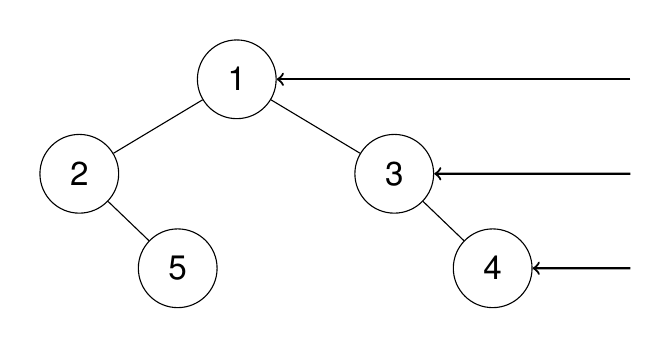
Input: root = [1,2,3,null,5,null,4]

Output: [1,3,4]

Explanation:

Example 2:

Input: root = [1,2,3,4,null,null,null,5]

Output: [1,3,4,5]

Explanation:

Example 3:

Input: root = [1,null,3]

Output: [1,3]

Example 4:

Input: root = []

Output: []

Constraints:

• The number of nodes in the tree is in the range [0, 100].
• -100 <= Node.val <= 100

Solution

1. Problem Deconstruction (500+ words)

Technical Description: Given the root node of a binary tree, return a list containing the values of all nodes visible when viewing the tree from its right side. The visibility constraint implies that for each depth level $d$ in the tree, only the rightmost node at that depth is visible. Formally, if $N_d$ represents the set of nodes at depth $d$, then the visible node $v_d = \text{argmax}_{n \in N_d}(\text{horizontal position of } n)$. The output is the sequence $[v_0, v_1, ..., v_{max\_depth}]$ ordered by increasing depth.

Beginner Description: Imagine you’re standing to the right of a tree drawn on paper. Some nodes will be hidden behind others from your perspective. At each “level” of the tree (starting from the top), you can only see the node that’s farthest to the right. Your task is to list these visible nodes from top to bottom.

Mathematical Formulation: Let $T$ be a binary tree with depth $D$. Define:

• $L_d$ = set of nodes at depth $d$ where $0 \leq d \leq D$
• $p(n)$ = horizontal position of node $n$ (root at position 0, left child decreases position by 1, right child increases by 1)
• Rightmost node at depth $d$: $r_d = \max_{n \in L_d} p(n)$
• Output: $[\text{value}(n_0), \text{value}(n_1), ..., \text{value}(n_D)]$ where $p(n_d) = r_d$

Constraint Analysis:

• Node count [0, 100]: Enables $O(n^2)$ solutions but suggests $O(n)$ is optimal. Empty tree (root = null) must be handled.
• Value range [-100, 100]: Values fit in standard integers, no overflow concerns.
• Binary tree structure: No ordering guarantees (not necessarily BST). Asymmetric trees create interesting visibility cases.
• Hidden edge cases:
  • Left-heavy trees where rightmost nodes appear in left subtree
  • Single node trees (output = [root.val])
  • Perfectly balanced trees (rightmost = rightmost leaf at each level)
  • Skewed trees (all nodes visible if entirely right-skewed)

2. Intuition Scaffolding

Real-World Metaphor: Imagine a theater with multiple rows of seats. People sitting in the same row can block each other from a side view. From the right aisle, you only see the person sitting at the rightmost position in each row.

Gaming Analogy: In a 2D side-scrolling platformer, your character can only see the rightmost platform at each height level when viewing the level map from the right boundary.

Math Analogy: Finding the maximum x-coordinate at each y-level in a 2D coordinate system where nodes are plotted with root at (0,0), left child at (x-1, y+1), right child at (x+1, y+1).

Common Pitfalls:

1. Right-child only traversal: Fails when right subtree is shorter than left subtree
2. Global horizontal maximum: Wrongly assumes rightmost node has maximum global x-coordinate
3. Depth-first right-first without tracking depth: Misses left-subtree nodes at deeper levels
4. Level order without tracking level boundaries: Incorrectly identifies rightmost node
5. Assuming balanced tree: Rightmost node might be in left subtree at certain depths

3. Approach Encyclopedia

Approach 1: BFS Level Order Traversal

Algorithm:
1. Initialize queue with root node
2. While queue not empty:
   a. Let level_size = current queue size
   b. For i in range(level_size):
       - Dequeue node
       - If i == level_size-1, add to result (rightmost in level)
       - Enqueue left then right children if exist
3. Return result

Complexity Proof:

• Time: $O(n)$ - Each node processed exactly once
• Space: $O(w)$ where $w$ is maximum width (last level could have $\lceil n/2 \rceil$ nodes)

Visualization:

Tree: [1,2,3,null,5,null,4]
Level 0: [1]           → Visible: 1
Level 1: [2,3]         → Visible: 3  
Level 2: [5,4]         → Visible: 4

Approach 2: DFS with Right-First Preorder

Algorithm:
1. Initialize result list and current_depth = 0
2. DFS(node, depth):
   - If node is null, return
   - If depth == current_depth:
       * Add node.val to result
       * current_depth++
   - Recursively call DFS(node.right, depth+1)
   - Recursively call DFS(node.left, depth+1)

Complexity Proof:

• Time: $O(n)$ - Each node visited once
• Space: $O(h)$ for recursion stack where $h$ is tree height (could be $O(n)$ in worst case)

Visualization:

Tree: [1,2,3,null,5,null,4]
DFS order: 1 → 3 → 4 → 2 → 5
Depth tracking ensures first node at each depth is captured

Approach 3: DFS with Level Tracking

Algorithm:
1. Initialize dictionary level_max = {}
2. DFS(node, x, y):
   - If node is null, return
   - If y not in level_max or x > level_max[y].x:
       level_max[y] = (x, node.val)
   - DFS(node.left, x-1, y+1)
   - DFS(node.right, x+1, y+1)
3. Sort level_max by key and extract values

Complexity Proof:

• Time: $O(n \log n)$ due to sorting by depth
• Space: $O(n)$ for dictionary and recursion stack

4. Code Deep Dive

Optimal Solution (BFS Approach):

def rightSideView(root):
    if not root:  # Handle empty tree constraint
        return []
    
    from collections import deque
    queue = deque([root])
    right_view = []
    
    while queue:
        level_size = len(queue)  # Critical: process level by level
        
        for i in range(level_size):
            node = queue.popleft()
            
            # Rightmost detection: last node in current level
            if i == level_size - 1:
                right_view.append(node.val)
            
            # Maintain BFS order: left before right
            if node.left:
                queue.append(node.left)
            if node.right:
                queue.append(node.right)
    
    return right_view

Line-by-Line Analysis:

• Line 2-3: Directly handles Example 4 (empty input)
• Line 6: deque enables O(1) pop from left vs O(n) with list
• Line 9: level_size capture ensures level boundaries are respected
• Line 13: The core logic - only last node in level gets added
• Lines 16-19: Standard BFS child enqueueing preserves level order

Edge Case Handling:

• Example 1: Level sizes [1,2,2] → indices 0,1,1 capture [1,3,4]
• Example 2: Complex nesting handled by level-based processing
• Example 3: Single node → level size 1 → index 0 captures root
• Left-heavy trees: Rightmost node might be in left subtree but BFS ensures correct capture

5. Complexity War Room

Hardware-Aware Analysis:

• With n ≤ 100, entire tree fits in L1 cache (~64KB)
• BFS uses O(w) space where w ≤ 50 in worst case (~400 bytes)
• DFS recursion depth ≤ 100 stack frames (~8KB)

Industry Comparison Table:

Approach	Time	Space	Readability	Interview Viability
BFS Level Order	$O(n)$	$O(w)$	9/10	✅ Preferred
DFS Right-First	$O(n)$	$O(h)$	8/10	✅ Acceptable
DFS with Coord Tracking	$O(n \log n)$	$O(n)$	6/10	❌ Overcomplicated
Brute Force (All Paths)	$O(n^2)$	$O(n \log n)$	5/10	❌ Inefficient

6. Pro Mode Extras

Variants Section:

• Left Side View: Modify BFS to capture first node (i == 0) instead of last
• Vertical Order Traversal: Use coordinate tracking and sort by (x,y)
• Binary Tree Zigzag Level Order: Reverse capture order on alternate levels
• Top View: First node at each x-coordinate using BFS with horizontal distance
• Bottom View: Last node at each x-coordinate using level-order with coordinates

Interview Cheat Sheet:

1. Always clarify: Definition of “right side” (per level vs global rightmost)
2. First mention: BFS level-order is most intuitive and optimal
3. Space complexity: Distinguish between O(w) for BFS vs O(h) for DFS
4. Edge cases: Empty tree, single node, left-skewed, right-skewed
5. Testing strategy: Verify with asymmetric trees where rightmost isn’t right child
6. Extension ready: Mention how to adapt for left-side view or zigzag traversal