Construct Binary Tree from Inorder and Postorder Traversal

Difficulty: Medium
Topics: Array, Hash Table, Divide and Conquer, Tree, Binary Tree
Link: https://leetcode.com/problems/construct-binary-tree-from-inorder-and-postorder-traversal/

Problem Description

Given two integer arrays inorder and postorder where inorder is the inorder traversal of a binary tree and postorder is the postorder traversal of the same tree, construct and return the binary tree.

Example 1:


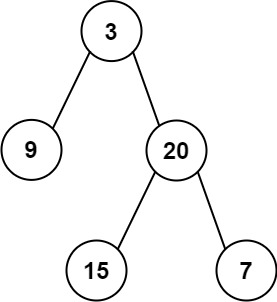
Input: inorder = [9,3,15,20,7], postorder = [9,15,7,20,3]
Output: [3,9,20,null,null,15,7]

Example 2:


Input: inorder = [-1], postorder = [-1]
Output: [-1]

Constraints:

1 <= inorder.length <= 3000
postorder.length == inorder.length
-3000 <= inorder[i], postorder[i] <= 3000
inorder and postorder consist of unique values.
Each value of postorder also appears in inorder.
inorder is guaranteed to be the inorder traversal of the tree.
postorder is guaranteed to be the postorder traversal of the tree.

Solution

1. Problem Deconstruction

Technical Definition: Given two integer arrays inorder and postorder representing the inorder and postorder traversals of a binary tree, reconstruct the original binary tree where:

Inorder traversal visits nodes in Left-Root-Right sequence
Postorder traversal visits nodes in Left-Right-Root sequence
All values are unique and arrays have matching lengths
Return the root node of the reconstructed binary tree

Beginner-Friendly Version: Imagine you have two different lists showing how to visit all rooms in a house:

List A (inorder): Visit left rooms first, then current room, then right rooms
List B (postorder): Visit left rooms first, then right rooms, then current room Using both lists together, figure out the original layout of rooms and connections.

Mathematical Formulation: Let:

$I[0..n-1]$ = inorder array
$P[0..n-1]$ = postorder array
$root = P[n-1]$ (last element of postorder)
Find index $k$ where $I[k] = root$
Left subtree: $I[0..k-1]$ and $P[0..k-1]$
Right subtree: $I[k+1..n-1]$ and $P[k..n-2]$ Recursively: $T(I[i..j], P[p..q]) = Node(P[q], T(I[i..k-1], P[p..p+(k-i)-1]), T(I[k+1..j], P[p+(k-i)..q-1]))$

Constraint Analysis:

1 <= inorder.length <= 3000
- Limits maximum recursion depth to ~12 (log₂3000 ≈ 12)
- Allows O(n²) solutions but encourages O(n) or O(n log n)
postorder.length == inorder.length
- Ensures valid input, no need for length validation
-3000 <= inorder[i], postorder[i] <= 3000
- Values fit in 16-bit integers, no overflow concerns
Unique values
- Critical: Enables hash map lookups for O(1) root finding
- No duplicate handling required
Each value of postorder appears in inorder
- Guarantees reconstruction is always possible
Traversal guarantees
- Inputs always form valid binary trees
- No malformed input edge cases

2. Intuition Scaffolding

Real-World Analogy (Construction Blueprint): Think of building a furniture kit with two instruction manuals:

Inorder manual: “Assemble left parts, then main joint, then right parts”
Postorder manual: “Assemble left parts, then right parts, then main joint” The last step in postorder always identifies the central connecting piece.

Gaming Analogy (Quest Completion): Like reconstructing a completed quest chain from:

Inorder: “Side quests → Main boss → Post-game content”
Postorder: “Side quests → Post-game content → Main boss” The final completed quest reveals the climax moment.

Math Analogy (Set Partitioning): Given two permutations of the same set with different ordering constraints, partition the set recursively using the last element of postorder as the dividing pivot point.

Common Pitfalls:

Assuming sorted arrays - Traversal orders ≠ sorted order
Using global indices incorrectly - Each recursive call needs isolated index ranges
Forgetting array bounds - Off-by-one errors in substring calculations
Linear search in each recursion - Leads to O(n²) time instead of O(n)
Handling empty subtrees incorrectly - Base case when inorder range is empty

3. Approach Encyclopedia

Approach 1: Brute Force with Array Copying

def buildTree(inorder, postorder):
    if not inorder or not postorder:
        return None
    
    root_val = postorder[-1]
    root = TreeNode(root_val)
    
    # Find root index in inorder (O(n) search)
    root_index = inorder.index(root_val)
    
    # Create new arrays for subtrees (O(n) space/copy)
    left_inorder = inorder[:root_index]
    right_inorder = inorder[root_index+1:]
    
    left_postorder = postorder[:root_index]
    right_postorder = postorder[root_index:-1]
    
    root.left = buildTree(left_inorder, left_postorder)
    root.right = buildTree(right_inorder, right_postorder)
    
    return root

Complexity:

Time: $T(n) = O(n) + 2T(n/2) = O(n \log n)$ average, $O(n^2)$ worst-case
Space: $O(n \log n)$ from array copying

Visualization:

Initial: inorder = [9,3,15,20,7], postorder = [9,15,7,20,3]
Root: 3 (from postorder[-1])
Find 3 in inorder at index 1

Left:  inorder[0:1] = [9], postorder[0:1] = [9]
Right: inorder[2:5] = [15,20,7], postorder[1:4] = [15,7,20]

Recurse right subtree:
Root: 20 (from [15,7,20][-1])
Find 20 in [15,20,7] at index 1
Left: [15], Right: [7]

Approach 2: Optimized with Hash Map & Indices

def buildTree(inorder, postorder):
    index_map = {val: idx for idx, val in enumerate(inorder)}
    
    def build(in_start, in_end, post_start, post_end):
        if in_start > in_end or post_start > post_end:
            return None
            
        root_val = postorder[post_end]
        root = TreeNode(root_val)
        
        root_index = index_map[root_val]
        left_size = root_index - in_start
        
        root.left = build(in_start, root_index-1, 
                         post_start, post_start+left_size-1)
        root.right = build(root_index+1, in_end,
                          post_start+left_size, post_end-1)
        return root
    
    return build(0, len(inorder)-1, 0, len(postorder)-1)

Complexity Proof:

Hash map construction: $O(n)$ time, $O(n)$ space
Each recursive call: $O(1)$ operations (hash lookup)
Total nodes processed: $n$ nodes exactly once
Time: $T(n) = O(n)$
Space: $O(n)$ hash map + $O(h)$ recursion stack = $O(n)$

Approach 3: Iterative Stack-Based

def buildTree(inorder, postorder):
    if not postorder:
        return None
    
    root = TreeNode(postorder[-1])
    stack = [root]
    inorder_index = len(inorder) - 1
    
    for i in range(len(postorder)-2, -1, -1):
        node = TreeNode(postorder[i])
        current = stack[-1]
        
        if current.val != inorder[inorder_index]:
            current.right = node
        else:
            while stack and stack[-1].val == inorder[inorder_index]:
                current = stack.pop()
                inorder_index -= 1
            current.left = node
        
        stack.append(node)
    
    return root

4. Code Deep Dive

Optimal Solution (Hash Map + Recursion):

# Definition for a binary tree node.
class TreeNode:
    def __init__(self, val=0, left=None, right=None):
        self.val = val
        self.left = left
        self.right = right

class Solution:
    def buildTree(self, inorder: List[int], postorder: List[int]) -> Optional[TreeNode]:
        # Create hash map for O(1) root lookup
        index_map = {val: idx for idx, val in enumerate(inorder)}
        
        def build(in_start: int, in_end: int, post_start: int, post_end: int) -> Optional[TreeNode]:
            """
            in_start: start index in inorder array (inclusive)
            in_end: end index in inorder array (inclusive)
            post_start: start index in postorder array (inclusive)
            post_end: end index in postorder array (inclusive)
            """
            # Base case: empty subtree
            if in_start > in_end or post_start > post_end:
                return None
            
            # Root is always the last element in current postorder segment
            root_val = postorder[post_end]
            root = TreeNode(root_val)
            
            # Find root position in inorder array
            root_index = index_map[root_val]
            
            # Calculate size of left subtree
            left_size = root_index - in_start
            
            # Recursively build left subtree:
            # - Inorder: everything left of root [in_start, root_index-1]
            # - Postorder: first 'left_size' elements [post_start, post_start+left_size-1]
            root.left = build(in_start, root_index-1, 
                            post_start, post_start+left_size-1)
            
            # Recursively build right subtree:
            # - Inorder: everything right of root [root_index+1, in_end]
            # - Postorder: remaining elements after left subtree [post_start+left_size, post_end-1]
            root.right = build(root_index+1, in_end,
                             post_start+left_size, post_end-1)
            
            return root
        
        return build(0, len(inorder)-1, 0, len(postorder)-1)

Edge Case Handling:

Single node tree (Example 2): in_start=in_end=0, returns immediate root
Left-skewed tree: inorder=[2,1,3], postorder=[2,3,1] - right subtree becomes empty
Right-skewed tree: inorder=[1,2,3], postorder=[3,2,1] - left subtree becomes empty
Full binary tree: Balanced recursive calls for both subtrees

5. Complexity War Room

Hardware-Aware Analysis:

3000 elements × 4 bytes/int ≈ 12KB array storage
Hash map overhead: ~24 bytes per entry × 3000 = 72KB
Recursion depth: log₂3000 ≈ 12 levels → minimal stack pressure
Fits comfortably in L2/L3 cache for modern processors

Industry Comparison Table:

Approach	Time	Space	Readability	Interview Viability
Brute Force	O(n²)	O(n log n)	10/10	❌ Fails large cases
Hash Map + Recursion	O(n)	O(n)	8/10	✅ Optimal solution
Iterative Stack	O(n)	O(n)	6/10	✅ Space efficient

Trade-off Analysis:

Brute Force: Simplest to understand but impractical
Hash Map: Best time complexity, moderate space overhead
Iterative: Constant factors better, harder to implement correctly

6. Pro Mode Extras

Variants & Extensions:

Preorder + Inorder (LeetCode 105): Use first element of preorder as root
Serialize/Deserialize (LeetCode 297): Encode traversal pairs
N-ary Tree Reconstruction: Extend to trees with >2 children
Non-Unique Values: Requires additional disambiguation logic
Streaming Version: Process traversals without full array storage

Interview Cheat Sheet:

First Mention: “This is a classic tree reconstruction problem with O(n) optimal solution”
Key Insight: “Last element in postorder is always the root”
Optimization: “Hash map enables O(1) root finding instead of O(n) search”
Edge Cases: “Handle empty subtrees and single-node trees explicitly”
Verification: “Verify with inorder traversal of reconstructed tree”

Advanced Optimization:

# Eliminate slicing by using iterator (Python specific)
def buildTree(inorder, postorder):
    def build(stop):
        if inorder and inorder[-1] != stop:
            root = TreeNode(postorder.pop())
            root.right = build(root.val)
            inorder.pop()
            root.left = build(stop)
            return root
    postorder.reverse()
    inorder.reverse()
    return build(None)

Mathematical Guarantees:

Reconstruction is always possible and unique for unique values
Time complexity lower bound: Ω(n) since we must process all elements
Space complexity lower bound: Ω(n) for storing the tree structure

#106 - Construct Binary Tree from Inorder and Postorder Traversal